excel-lambda-FREQ.SIMPLE – create a simple frequency table in Excel with one function

The gist for this lambda function can be found here.

The goal

The goal in this post is:

Create a simple frequency table in Excel with one function

A solution

Here’s a lambda function called FREQ.SIMPLE:

FREQ.SIMPLE =LAMBDA(data,
    LET(
        d, INDEX(data,,1),
        u,  UNIQUE(d),
        X,  N(u = TRANSPOSE(d)),
        Y,  SEQUENCE(ROWS(d), 1, 1, 0),
        mp, MMULT(X,Y),
        c,  CHOOSE({1,2}, u, mp),
        SORT(c, 2, -1)
    )
);

FREQ.SIMPLE has one parameter and as such accepts one argument.

1. data – a single-column array of data. This is usually a column of text values with some duplication and we want to count the occurrences of each unique value in the column.

How it works

Here’s how it works:

This is a very simple function, written initially to be used by other functions, such as KNN.

If you’d like to use it, you can grab the code from the gist linked at the top of this page. 

Let’s break it down

As a reminder, this function is defined as:

FREQ.SIMPLE =LAMBDA(data,
    LET(
        d, INDEX(data,,1),
        u,  UNIQUE(d),
        X,  N(u = TRANSPOSE(d)),
        Y,  SEQUENCE(ROWS(d), 1, 1, 0),
        mp, MMULT(X,Y),
        c,  CHOOSE({1,2}, u, mp),
        SORT(c, 2, -1)
    )
);

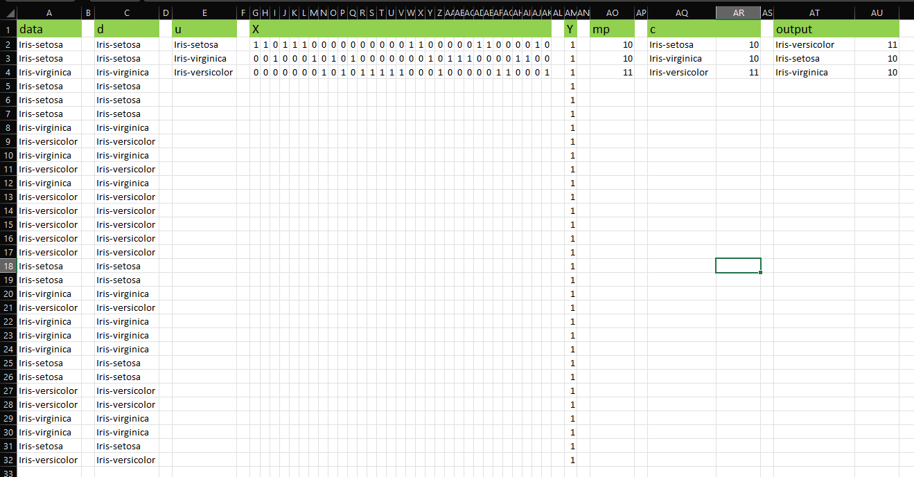
We define some names with bound values:

• d – here we use INDEX to take the first column of the data parameter, in case more than one column has been selected while calling the function. 
• u – creates an array of the unique values found in d.
• X – creates an array that is ROWS(data) columns wide and ROWS(UNIQUE(data)) rows tall. The array is populated with either 1 or 0. A 1 means that the value in that row of d (the data) of which that column is the transpose, matches the value in the same row of the unique list of values represented by u. This restructuring of data is necessary to use the MMULT function in a following step. 
• Y – produces an array the same length as d with 1 in every row.
• mp – returns the matrix product of X and Y. The net result is that we have a sum of the 1s in X for each unique value in u. 
• c – here we combine the unique text value in u with their corresponding counts in mp. This is now a two-column array with ROWS(u) rows.
• Finally, we SORT the array c in descending order on column 2. The net result is those unique values with the highest frequency are at the top of the table.

This is what each name contains:

In summary

We saw how to create a simple frequency table in Excel with one function.

We restructured an array of values to use matrix multiplication to count occurrences of unique values in a column.

We used the SORT function to sort a 2-column array in descending order on the second column.