Use XLOOKUP and XMATCH with regular expressions (regex)

Posted on 2024-06-132024-06-13 by OP

The Excel team introduced support for regular expressions in May 2024 with three new functions

REGEXREPLACE, which ‘allows you to replace text from a string with another string, based on a supplied regular expression (“regex”)’.
REGEXEXTRACT, which ‘allows you to extract text from a string based on a supplied regular expression. You can extract the first match, all matches or capturing groups from the first match’.
REGEXTEST, which ‘allows you to check whether any part of supplied text matches a regular expression (“regex”). It will return TRUE if there is a match and FALSE if there is not’.

The functions were announced in this post on the Microsoft 365 Insiders blog.

As well as these new functions, we learned that we will be able to use regular expressions with XLOOKUP and XMATCH in the near future.

Regex coming soon to XLOOKUP and XMATCH

We will also be introducing a way to use regex within XLOOKUP and XMATCH, via a new option for their ‘match mode’ arguments. The regex pattern will be supplied as the ‘lookup value’.

This will be available for you to try in Beta soon, at which point we’ll update this blog post with more details.

While we wait for that, we can mimic that functionality with lambda functions!

XMATCH.NEW

XMATCH.NEW = LAMBDA(lookup_value,lookup_array,[match_mode],[search_mode],
    IF(
        match_mode=3, // use regex
        FILTER(SEQUENCE(ROWS(TOCOL(lookup_array))),REGEXTEST(lookup_array,lookup_value)),
        XMATCH(lookup_value, lookup_array, match_mode, search_mode)
    )
);

XMATCH.NEW works very similarly to XMATCH. In fact, unless we pass match_mode=3, it works identically to XMATCH.

If we pass match_mode=3, XMATCH.NEW interprets the lookup_value as a regex pattern. The pattern is tested against the lookup_array using REGEXTEST. This returns an array of TRUE/FALSE values. This array, or mask if you prefer, is passed as the include argument in the FILTER function, where the array being filtered is the positional indices of the lookup_array – SEQUENCE(ROWS(TOCOL(lookup_array))).

As a simple example, let’s use this pattern ^(?![^@\s]+@[^@\s]+.[^@\s]{2,}\s*$).+$ to find the positional indices of the invalid email addresses in this made-up dataset.

The pattern is passed as the lookup_value, the array is the range of email addresses in column C, and the match_mode is set to 3. So, the function returns the indices (shown in column G) of those rows where REGEXTEST returns TRUE (shown in column F). Whereas XMATCH only returns the first index of a valid match, XMATCH.NEW with match_mode 3 will return all matching indices.

XLOOKUP.NEW

XLOOKUP.NEW = LAMBDA(lookup_value,lookup_array,return_array,
                    [if_not_found],[match_mode],[search_mode],
    IF(
        match_mode=3, // use regex
        IFERROR(
            FILTER(return_array,REGEXTEST(lookup_array,lookup_value)),
            IF(ISOMITTED(if_not_found),#N/A,if_not_found)
        ),
        XLOOKUP(lookup_value,lookup_array,return_array,if_not_found,match_mode,search_mode)
    )
);

XLOOKUP.NEW will behave identically to XLOOKUP unless we pass match_mode=3, in which case the pattern in lookup_value will be used in REGEXTEST to build an array of TRUE/FALSE values which are passed as the include parameter in FILTER. This time, the array being filtered will be return_array, returning the matching rows. If this filter operation returns an error, the function returns to the spreadsheet the argument supplied to the if_not_found parameter, or #N/A if no such argument was provided.

Let’s use the same invalid email address pattern to filter the data for rows with invalid email addresses:

The pattern is passed as the lookup_value, the lookup_array is the range of email addresses in column C, the return_array is the range of data in columns A to E, and the match_mode is set to 3. So, the function returns those rows where REGEXTEST returns TRUE (shown in column F).

Simple!

CONCLUSION

While we wait for the official update that will allow us to use regular expressions with XLOOKUP and XMATCH, we can make some simple LAMBDA functions that will mimic this behavior, and start to practice our regular expressions now!

Click here for another post about regular expressions, and why “just get it from AI” is not going to be good enough.

Unfold a list with this new function

Posted on 2024-05-102024-05-10 by OP

In this post you’ll learn to unfold a list from a value with a recursion wrapper called LIST.UNFOLD.

INTRODUCTION

In Excel as in many other languages, we can use REDUCE to reduce (or fold) a list into a single value. We iterate over the list, and at each element apply a function. The result of that function becomes what’s known as an accumulator. This accumulator created from applying the function to one element is passed as an argument to the same function when it is applied to the next element. This continues until the last element of the list is reached, at which point the accumulator becomes the result.

So, with REDUCE, we can create a single value from a list and a function.

In some languages this operation is known as “folding”. In fact, I talked about that in an earlier post. It turns out that in several functional programming languages have built-in capability to do the opposite of the reduce (or fold) operation.

Let’s look at List.unfold from F#. Here’s the example from the documentation:

|> List.unfold (fun state -> if state > 100 then None else Some (state, state * 2))

Both Some and None are part of what’s known as an Option type in F#. They are used to safely handle values that might or might not exist. When the if statement returns true, i.e. when state is greater than 100, the return of None is an error-safe way to indicate that there are no more values to add to the list. This is essentially the exit condition to tell List.unfold to stop. If state is less than or equal to 100, Some (state, state * 2) creates a tuple whose first element is the next element to be added to the list. The second element is the new value of state to pass to the next iteration of the generator function. So, this is a concise way of using recursion to generate a list and one of the many reasons why F# is a great language!

Reading this you may be thinking… hey, is that why we have List.Generate in Power Query?

Yes. Yes, it is.

In fact, my observation is that List.Generate encapsulates the functionality of List.unfold and adds additional functionality to handle common data mashup use cases that might be needed in the realms of Excel, Power BI et al.

Anyway, we’re getting off track! Let’s look at LIST.UNFOLD as an Excel LAMBDA function!

LIST.UNFOLD

Here’s the code for LIST.UNFOLD:

LIST.UNFOLD = LAMBDA(generator_function, 
    LAMBDA(value,
        LET(
            _result, generator_function(value),
            IF(ISNA(@TAKE(_result,-1, 1)), value, LIST.UNFOLD(generator_function)(_result))
        )
    )
);

Looks simple, right? And it is! I’ll break it down for you in a minute, but let’s talk about the signature. There are two required (and curried) parameters. The reason for that will become clear shortly.

generator_function – this is the function that will take the current state of the list and produce a new value to be added. This function can be very simple or incredibly complex. The requirement placed on this function is that it has one parameter. There is no requirement on the type of that parameter.
value – this is the current state of the list. When we call LIST.UNFOLD, we’ll give this inner lambda a seed value to get started on, and as the function recurses, the list being created will be passed into this parameter.

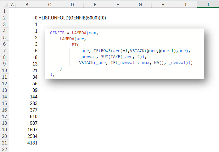
Here’s an example of how LIST.UNFOLD works:

GENFIB is a general implementation of a Fibonacci-like sequence. This function calculates the new value as the sum of the previous two values. It then stacks the new value underneath the previous values. Here’s the code for GENFIB:

GENFIB = LAMBDA(max,
    LAMBDA(arr, 
        LET(
            _arr, IF(ROWS(arr)=1,VSTACK(@arr,@arr+1),arr),
            _newval, SUM(TAKE(_arr,-2)), 
            VSTACK(_arr, IF(_newval > max, NA(), _newval)))
    )
);

The important thing here is that we can configure the exit condition by passing the first parameter as the value which will serve as an exit condition for the function. So this:

GENFIB(5000)

Returns this:

    LAMBDA(arr, 
        LET(
            _arr, IF(ROWS(arr)=1,VSTACK(@arr,@arr+1),arr),
            _newval, SUM(TAKE(_arr,-2)), 
            VSTACK(_arr, IF(_newval > 5000, NA(), _newval)))
    )

Now we can see that if the _newval (state) is greater than 5000, the function will stack NA() to the bottom of the list. This is a design decision I’ve made for LIST.UNFOLD. When LIST.UNFOLD encounters an NA() at the bottom of the list, it will stop. So any function passed to LIST.UNFOLD must use this fact to control the exit condition.

One thing to note about GENFIB itself is that it is not a recursive function. All it does is calculate one value. The recursion is handled by LIST.UNFOLD. This is a way to remove the difficult part of the programming from the logic of the sequence and re-use it whenever it’s needed.

Without further ado, let’s take a close look at how LIST.UNFOLD works!

BREAKDOWN

For reference, here’s the code for LIST.UNFOLD again. I’ve included the code for GENFIB as it may be helpful in the following explanation.

LIST.UNFOLD = LAMBDA(generator_function, 
    LAMBDA(value,
        LET(
            _result, generator_function(value),
            IF(ISNA(@TAKE(_result,-1, 1)), value, LIST.UNFOLD(generator_function)(_result))
        )
    )
);

GENFIB = LAMBDA(max,
    LAMBDA(arr, 
        LET(
            _arr, IF(ROWS(arr)=1,VSTACK(@arr,@arr+1),arr),
            _newval, SUM(TAKE(_arr,-2)), 
            VSTACK(_arr, IF(_newval > max, NA(), _newval)))
    )
);

So, we pass a generator_function into the outer lambda of LIST.UNFOLD. An example is GENFIB(5000) which returns the function discussed above:

=LIST.UNFOLD(GENFIB(5000))

That returns this inner function:

    LAMBDA(value,
        LET(
            _result, generator_function(value),
            IF(ISNA(@TAKE(_result,-1, 1)), value, LIST.UNFOLD(generator_function)(_result))
        )
    )

Where generator_function is:

    LAMBDA(arr, 
        LET(
            _arr, IF(ROWS(arr)=1,VSTACK(@arr,@arr+1),arr),
            _newval, SUM(TAKE(_arr,-2)), 
            VSTACK(_arr, IF(_newval > 5000, NA(), _newval)))
    )

When you expand all of this, that small line has actually created this function!

UNFOLD.GENFIB5000 = 
    LAMBDA(value,
            LET(
                generator_function, 
                    LAMBDA(arr, 
                        LET(
                            _arr, IF(ROWS(arr)=1,VSTACK(@arr,@arr+1),arr),
                            _newval, SUM(TAKE(_arr,-2)), 
                            VSTACK(_arr, IF(_newval > 5000, NA(), _newval)))
                    ),
                _result, generator_function(value),
                IF(ISNA(@TAKE(_result,-1, 1)), value, LIST.UNFOLD(generator_function)(_result))
            )
        );

Which is part of the reason I wanted to put the recursion logic inside LIST.UNFOLD. Anyway, let’s get back on track. Here’s LIST.UNFOLD again.

LIST.UNFOLD = LAMBDA(generator_function, 
    LAMBDA(value,
        LET(
            _result, generator_function(value),
            IF(ISNA(@TAKE(_result,-1, 1)), value, LIST.UNFOLD(generator_function)(_result))
        )
    )
);

_result is the result of whatever generator_function produces when we give it value.

An example:

=LIST.UNFOLD(GENFIB(5000))(0)

This function passes 0 into the generator_function GENFIB(5000).

    LAMBDA(arr, 
        LET(
            _arr, IF(ROWS(arr)=1,VSTACK(@arr,@arr+1),arr),
            _newval, SUM(TAKE(_arr,-2)), 
            VSTACK(_arr, IF(_newval > 5000, NA(), _newval)))
    )

So 0 is arr. And since ROWS(0)=1, this GENFIB function assigns VSTACK(0, 0+1) to _arr. This is important because a Fibonacci-like calculation requires two values to calculate the next value. The design choice here is to say if this function has only been given one value, then we’ll just put the next integer after it and continue as if there were two values in the array originally.
_newval is then the sum of those two values. Finally, check if _newval is greater than 5000 and if it isn’t, return _arr with _newval stacked underneath.
This return value is, as mentioned, assigned to _result in LIST.UNFOLD:

LIST.UNFOLD = LAMBDA(generator_function, 
    LAMBDA(value,
        LET(
            _result, generator_function(value),
            IF(ISNA(@TAKE(_result,-1, 1)), value, LIST.UNFOLD(generator_function)(_result))
        )
    )
);

Passing 0 to value as we did means that _result will be {0; 1; 1} after the first iteration.

The next line of LIST.UNFOLD first checks if the last row in _result is NA(). If it is, LIST.UNFOLD exits and returns value (i.e. the state of the list after the previous iteration). If the value of the last row is not NA(), LIST.UNFOLD is called again, but this time _result is the new argument to value.
When value={0; 1; 1} in GENFIB, ROWS({0; 1; 1})=3, so _arr=arr and _newval=SUM(TAKE({0; 1; 1},-2))=SUM({1; 1})=2. Further, _newval is not greater than 5000, so the return value of the generator function is now VSTACK({0; 1; 1}, 2)={0; 1; 1; 2}, which becomes _result in UNFOLD.LIST, and so on and so forth until the exit condition is met!

The recursion, which is fairly standard behavior across the family of functions that produce sequences, is always handled in the same way, and so has been abstracted into the LIST.UNFOLD function. The real logic of what the syntax is is embedded in the generator function, which as I mentioned before, can be as simple or as complex as you like. Here are a few examples:

GEOMETRIC = LAMBDA(common_ratio, break_at, 
    LAMBDA(x, 
        LET(
            _newval, @TAKE(x,-1)*common_ratio, 
            VSTACK(x, IF(OR(AND(common_ratio<1,_newval<break_at),
                            AND(common_ratio>=1,_newval>break_at)), NA(), _newval))))
);

POWERSEQ = LAMBDA(power,ceiling,
    LAMBDA(x, LET(_newval, @TAKE(x,-1)^power, VSTACK(x,IF(_newval > ceiling, NA(), _newval))))
);

GENFIB = LAMBDA(max,
    LAMBDA(arr, 
        LET(
            _arr, IF(ROWS(arr)=1,VSTACK(@arr,@arr+1),arr),
            _newval, SUM(TAKE(_arr,-2)), 
            VSTACK(_arr, IF(_newval > max, NA(), _newval)))
    )
);

CATALAN =LAMBDA(max, mode, 
    LAMBDA(
        arr, 
        LET(
            _n, TAKE(arr,-1,-1), 
            _Cn, TAKE(arr,-1,1), 
            _newVal, _Cn * 2 * (2*_n + 1) / (_n + 2),
            VSTACK(arr, IF(
                IF(mode=0,_newVal,_n+2) > max
                , NA(), HSTACK(_newVal, _n + 1)))
        )
    )
);

These are somewhat trivial examples since, according to my 8-step process for writing recursive functions in Excel, they probably aren’t necessary.

However, I’d just like to remind you that recursion is either necessary for the program or for the programmer. If it makes the programming easier to understand, then use it!

SUMMARY

In this post we saw how to unfold a list with this new function – LIST.UNFOLD.

LIST.UNFOLD is a recursion wrapper for the family of functions that produce complex sequences. Like List.Generate in Power Query, and List.unfold in F#, we can pass a generator function to LIST.UNFOLD along with a seed value, to create a new list, making it equivalent to the reverse of REDUCE!

I hope you enjoyed reading about it and that it sparked some ideas. Let me know in the comments if you have any questions!

8-Step Process For Writing Recursive Functions in Excel

Posted on 2024-05-102024-05-10 by OP

1. Write a recursive function in Excel
2. Realize you could’ve done it with REDUCE
3. Write it with REDUCE
4. Realize you could’ve done it with dynamic arrays
5. Write it with dynamic arrays
6. Realize there’s already a built-in function to do it
7. Use the built-in function
8. 😐

Excel LAMBDA: simplified rolling aggregate of any function

Posted on 2024-01-042024-01-04 by OP

The gist for this lambda function can be found here.

Preface

This post is a follow up to an earlier post. I wrote the function described there in May of 2022, before I had access to functions like VSTACK and HSTACK and before I had a solid understanding of SCAN and REDUCE. As such, while it was fun to write and worked just fine, it was a monster of a function!

The recent release of the GROUPBY and PIVOTBY functions (described here) also came with a huge upgrade to the LAMBDA experience. To cut a long-story short, with this release, we are now able to pass native functions as arguments to other functions.

As a very simple example, where before we might have had to do this to calculate column totals for an array:

=BYCOL(my_array, LAMBDA(c, SUM(c)))

The upgrade means we can now do this instead:

=BYCOL(my_array, SUM)

In short, instead of having to wrap the SUM function in a LAMBDA for it to be accepted as an argument to BYCOL, we can now simply pass the SUM function itself and BYCOL will interpret it as “single argument function” and pass the only argument BYCOL creates – a column from the array – into SUM.

The goal

If we have a table of sales of a product where each row represents one month, then we might want to calculate – for each month – the rolling sum of sales over the most recent three months.

When we sum a variable over multiple rows like this, the rows we are summing over are referred to as a “window” on the data. So, functions that apply calculations over a rolling number of rows are referred to as “window functions”.

These window functions are available in almost all flavors of SQL.

They’re also available in the Python Pandas package. In Pandas, we can use window functions by making calls to rolling.

The goal here is to mimic the functionality seen in pd.rolling by providing a generic and dynamic interface for calculating rolling aggregates.

rolling.aggregate – a simplified solution

This is the lambda function rolling.aggregate. The intention is that you would use the function below in an Advanced Formula Environment module called ‘rolling’:

aggregate =LAMBDA(x,window,
  LAMBDA(function,
    LET(
      _i,SEQUENCE(ROWS(x)),
      MAP(_i,
        LAMBDA(b,
          IF(
              b < window,
              NA(),
              function(INDEX(x, b - window + 1, 1):INDEX(x, b, 1))
          )
        )
      )
    )
  )
);

As you can see, it’s significantly simpler than the earlier version. Here’s an example showing a rolling sum:

For a rolling average, we just pass a different aggregation function:

rolling.aggregate takes three parameters:

1. x – the single-column array of numbers over which we want to calculate rolling aggregates
2. window – an integer representing the size of the window, i.e. the number of most-recent rows ending in the current row, that defines the window for the aggregate that will be displayed on the current row of the output array
3. function – a function with no more than one required argument that produces a scalar. For example, SUM, AVERAGE, MIN, MAX, STDEV.S, etc or a custom function such as:

=LAMBDA(x, TRIM(TEXTJOIN(", ", FALSE, x)))

This latter function concatenates the most recent 5 values:

rolling.aggregate – how it works

For reference:

aggregate =LAMBDA(x,window,
  LAMBDA(function,
    LET(
      _i,SEQUENCE(ROWS(x)),
      MAP(_i,
        LAMBDA(b,
          IF(
              b < window,
              NA(),
              function(INDEX(x, b - window + 1, 1):INDEX(x, b, 1))
          )
        )
      )
    )
  )
);

The first thing to note is that this is a curried function. If you’re not sure what that means, you may want to watch this video:

If you don’t want to watch the video, a quick primer is that when we curry a function, we separate one or more parameters of a function into separate functions.

When working with Excel LAMBDA functions, we can tell that a function has been curried when the first word after a list of parameters is LAMBDA. This means that the return value of that function is a LAMBDA function.

In this example, we can think of the “outer function” as:

aggregate =LAMBDA(x,window,
  LAMBDA()
);

And the “inner function” as:

  LAMBDA(function,
    LET(
      _i,SEQUENCE(ROWS(x)),
      MAP(_i,
        LAMBDA(b,
          IF(
              b < window,
              NA(),
              function(INDEX(x, b - window + 1, 1):INDEX(x, b, 1))
          )
        )
      )
    )
  )

So, we pass two parameters to the outer function: x – a vector (1-dimensional array), and window – an integer describing the number of rows over which the function should be applied. The return value of the outer function is the inner function, initialized with the values of x and window.

Considering the examples in the images above, x is B2:B14 and window is 5. The return value from passing those arguments to the outer function is:

  LAMBDA(function,
    LET(
      _i,SEQUENCE(ROWS(B2:B14)),
      MAP(_i,
        LAMBDA(b,
          IF(
            b < 5,
            NA(),
            function(INDEX(B2:B14, b - 5 + 1, 1):INDEX(B2:B14, b, 1))
          )
        )
      )
    )
  )

Note that occurrences of x are replaced with the range address B2:B14, and occurrences of window are replaced with 5. This is now a function of one parameter – function – which accepts the aggregate functions described above.

We call this function by passing the aggregate function we want to apply to the vector in parentheses after the function.

To be more specific, this is equivalent to the inner function LAMBDA above:

=rolling.aggregate(B2:B14,5)

We can think of this as preparing a function to accept whatever aggregate function we want to use at any given moment. For example:

=rolling.aggregate(B2:B14,5)(SUM)
=rolling.aggregate(B2:B14,5)(AVERAGE)
=rolling.aggregate(B2:B14,5)(MAX)
=rolling.aggregate(B2:B14,5)(LAMBDA(x, TRIM(TEXTJOIN(", ", FALSE, x))))
etc

You may be wondering “Why would we need to curry this function when we can just as easily have a single function call with three parameters?” We could do this instead:

=rolling.aggregate(B2:B14,5,SUM)

The benefit of currying the function parameter into the inner function is that we can prepare the inner function once, and use it multiple times:

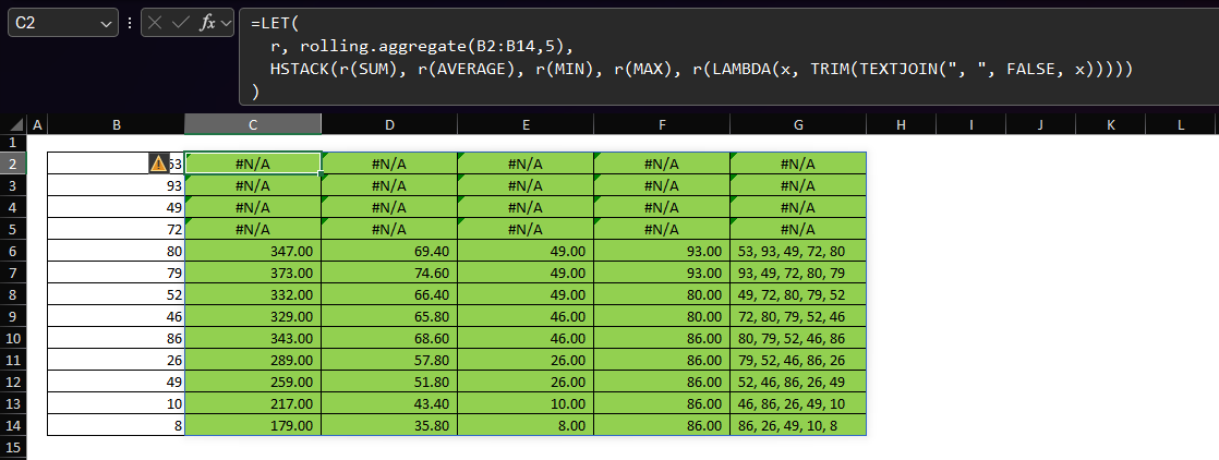
=LET(
  r, rolling.aggregate(B2:B14,5),
  HSTACK(r(SUM), r(AVERAGE), r(MIN), r(MAX), r(LAMBDA(x, TRIM(TEXTJOIN(", ", FALSE, x)))))
)

Which starts to make building multiple statistics over a pre-defined window size somewhat easy:

Let’s take a quick look at how the inner function works. As a reminder:

  LAMBDA(function,
    LET(
      _i,SEQUENCE(ROWS(x)),
      MAP(_i,
        LAMBDA(b,
          IF(
            b < window,
            NA(),
            function(INDEX(x, b - window + 1, 1):INDEX(x, b, 1))
          )
        )
      )
    )
  )

The body of the function uses LET:

_i – this is a sequence from 1 to the count of rows in x. In the examples used above, x is B2:B14, so ROWS(x) is 13 and SEQUENCE(ROWS(x)) is {1;2;3;4;5;6;7;8;9;10;11;12;13}

The return value of the LET call is a call to MAP. We are passing the array _i – the sequence {1;2;3;4;5;6;7;8;9;10;11;12;13} to the array1 parameter of MAP. Then, we are passing the following function to the lambda parameter of MAP:

LAMBDA(b, IF( b < window, NA(), function(INDEX(x, b - window + 1, 1):INDEX(x, b, 1)) ) )

This is just a function of one parameter – b – which represents one element from the sequence _i. The MAP function applies the expression beginning IF( b < window… to each value of b in _i.

The expression INDEX(x, b – window + 1, 1):INDEX(x, b, 1) builds a reference to the row of x that is window – 1 rows prior to the current value of b to the bth row in x. This is illustrated below using the ADDRESS function. Note that the row argument passed to ADDRESS is the same as the row argument passed to INDEX.

Then, the expression function(INDEX(x, b – window + 1, 1):INDEX(x, b, 1)) ) simply applies to the reference created with INDEX whatever function happens to be. For example, if function is SUM, then:

In summary

This post aimed to describe a simple but flexible way to create rolling aggregates using a custom curried lambda function.

Being able to pass native Excel functions (such as SUM, AVERAGE or MAX) as arguments to other functions allows us to create generic lambda functions whose result is controlled by a parameter.

Let me know in the comments if you have any questions about the post.

Breadth-first search using Excel

Posted on 2023-01-18 by OP

The code shown in this post can be found here.

What is breadth-first search?

Breadth-first search is a popular graph traversal algorithm. It can be used to find the shortest route between two nodes, or vertices, in a graph.

For a good primer on how this algorithm works, you can watch this video:

Put simply, breadth-first search, which for the remainder of this post I’ll refer to as BFS, uses a queue data structure to prioritize which nodes of the graph to visit next. The important thing to remember about a queue is that it is a first-in-first-out data structure (FIFO), which means that items added to the queue earlier are removed from the queue in the order they’re added.

Consider this graph where we want to find the shortest route from node A to node F:

We can represent this graph in Excel in several ways. Here’s one, which shows each node and the neighbors of that node:

BFS starts by adding node A to the queue.

Queue = {A}

We also initialize a secondary data structure, typically a dictionary or in Excel terms, an array, that keeps track of the nodes we have already visited along with where they were visited from. Because A was the start, we initialize it as follows:

Visited = {A: None}

The algorithm continues as follows:

First iteration

1. Dequeue an item from the queue.

This removes the left-most (first-in) node from the queue and makes it the current node. On the first iteration, this is just Node A. So:

Current node = A

2. Is the current node the goal?

If A = F, then exit the algorithm. Otherwise:

3. For each node adjacent to the current node

i.e., the yellow nodes B and C

Is the node under consideration in the visited array? If not: (a) add it to the queue and (b) add it to the visited array.

After the iteration, we have:

Queue = { B, C }

(because B was added to the queue, then C was added to the queue)

Visited = {A: None , B: A, C: A}

(because B and C were visited from A, in that order)

Represented in Excel, the state of the data at the end of the first iteration:

Second iteration

1. Dequeue an item from the queue.

This removes the left-most (first-in) node from the queue and makes it the current node. The left-most item in the queue is B, so:

Current node = B

2. Is the current node the goal?

If B = F, then exit the algorithm. Otherwise:

3. For each node adjacent to the current node

i.e., the yellow nodes D and E

Is the node under consideration in the visited array? If not: (a) add it to the queue and (b) add it to the visited array.

After the iteration, we have:

Queue = { C , D, E }

(because D was added to the queue, then E was added to the queue)

Visited = {A: None , B: A, C: A, D: B, E: B }

(because D and E were visited from B, in that order)

And in Excel, we have this:

And so on

The algorithm continues in in this way, successively adding items that haven’t yet been visited to the end of the queue and removing one item at a time from the front of the queue and checking if it’s the goal.

In the end, the visited array from this example looks like this:

At this point, the algorithm encounters node F and exits because it’s reached the goal. From this visited array, we can see that F was reached from C and C was reached from A, making the path from A to F:

A – C – F

Let’s see how we can automate this process with a lambda function or two.

The goal

Create lambda functions that will calculate a breadth-first search and return various artifacts to help with analysis of paths between nodes of a graph.

A solution

graph.breadth_first_search

All of the following functions I am using in a namespace called “graph”.

breadth_first_search = LAMBDA(queue, end, [visited], [iteration],
    LET(
        _iteration, IFOMITTED(iteration, 1, iteration + 1),
        _node, INDEX(TAKE(queue, 1), 1, 1),
        _visited, IFOMITTED(visited, HSTACK(_node, "None")),
        _is_undiscovered, LAMBDA(node, ISERROR(XMATCH(node, TAKE(_visited, , 1)))),
        _neighbors, graph.get_neighbors(_node),
        _end_is_neighbor, NOT(ISERROR(XMATCH(end, _neighbors))),
        _newqueue, 
        IF(
            OR(ISERROR(DROP(queue, 1))),
            _neighbors,
            REDUCE(
                DROP(queue, 1),
                _neighbors,
                LAMBDA(a, b, IF(_is_undiscovered(b), VSTACK(a, b), a))
            )
        ),
        
        _newvisited, REDUCE(
            _visited,
            _neighbors,
            LAMBDA(a, b, IF(_is_undiscovered(b), VSTACK(a, HSTACK(b, _node)), a))
        ),
        _result, IF(
            OR(_node = end, _end_is_neighbor),
            VSTACK(_visited, HSTACK(end, _node)),
            graph.breadth_first_search(_newqueue, end, _newvisited, _iteration)
        ),
        _result
    )
);

graph.breadth_first_search takes two required parameters:

queue – which is the state of the queue object during the iteration being passed to the function (this function is recursive). When called from the spreadsheet, the queue parameter is passed the “from” node – i.e. the start of the search. This is consistent with the initialization of the search as described above, where the start node is placed in the queue when the algorithm begins.
end – the goal node (i.e. the node we are searching for).

And two optional parameters, which are used by the recursion and generally do not need to be passed to the function when calling it from a spreadsheet:

[visited] – this is the current state of the visited array as described above. As the function iterates/searches, more and more nodes are added to the visited array.
[iteration] – this is a simple integer counter which keeps track of how many iterations have been used. I used it to help with debugging while writing the function.

The function defines names using LET:

_iteration – here we provide a default value of 1 for the optional [iteration] parameter, otherwise if [iteration] is passed to the function, we increment it by one, indicating that we have passed into a new iteration
_node – since BFS is a FIFO (first-in, first-out) function, we use TAKE(queue, 1) to take the first item from the queue. Since TAKE returns an array, and we need _node to be a single value and not a single-cell array, we use INDEX(arr,1,1) to convert it. _node is then the “current node” as described above.
_visited – here we are using a helper function I’ve called IFOMITTED, which replaces the oft-used pattern IF(ISOMITTED([optional parameter]),”some default”,[optional parameter])). So, here if the [visited] parameter is omitted from the function call, the default is to initialize it with HSTACK(_node, “None”), which is consistent with the explanation given above. As a side note, I’ve made a request to have a function called IFOMITTED added to Excel. I would really appreciate if you could go to the page and vote for the idea. The page is here. For now, the IFOMITTED function I’m using in this example is defined like this:

IFOMITTED = LAMBDA(arg, then, [else],
    LET(_else, IF(ISOMITTED(else), arg, else), IF(ISOMITTED(arg), then, _else))
);

_is_undiscovered – this embedded LAMBDA function checks if a node passed to it already exists in the first column of the _visited array. If it does not exist in that column, this function returns TRUE.
_neighbors – here we use a function called graph.get_neighbors to retrieve the nodes connected to the current node. I’ll first explain how that works before continuing with this explanation of graph.breadth_first_search.

graph.get_neighbors

data = Sheet1!A2:B4;

get_neighbors_fn = LAMBDA(data,
    LAMBDA(node,
        LET(
            _neighbors, INDEX(FILTER(TAKE(data, , -1), TAKE(data, , 1) = node), 1, 1),
            TEXTSPLIT(_neighbors, , ", ")
        )
    )
);

get_neighbors = graph.get_neighbors_fn(graph.data);

You can see that the get_neighbors function is calling graph.get_neighbors_fn(graph.data).

graph.data is a named range pointing to the data in the workbook that contains the graph definition.

When we pass the data to graph.get_neighbors_fn, it returns the inner function:

    LAMBDA(node,
        LET(
            _neighbors, INDEX(FILTER(TAKE(data, , -1), TAKE(data, , 1) = node), 1, 1),
            TEXTSPLIT(_neighbors, , ", ")
        )
    )

This inner function assumes the data are formatted as in the example above – two columns with the node in the first column and the neighbors of that node in the second column.

It filters the data to find the node passed to its parameter, returning the cell containing the neighbors of that node, then splits the comma-separated neighbors into an array.

The array of neighbors is then returned to the calling function.

The reason I separated this “get neighbors” process into a different function was so that the breadth_first_search function could be used with other functions to return the neighbors of a given node, which may then be defined on graph data structured in a different way to this example.

Anyway, let’s continue looking at breadth-first search.

graph.breadth_first_search (continued)

As a reminder, here’s the code again:

breadth_first_search = LAMBDA(queue, end, [visited], [iteration],
    LET(
        _iteration, IFOMITTED(iteration, 1, iteration + 1),
        _node, INDEX(TAKE(queue, 1), 1, 1),
        _visited, IFOMITTED(visited, HSTACK(_node, "None")),
        _is_undiscovered, LAMBDA(node, ISERROR(XMATCH(node, TAKE(_visited, , 1)))),
        _neighbors, graph.get_neighbors(_node),
        _end_is_neighbor, NOT(ISERROR(XMATCH(end, _neighbors))),
        _newqueue, 
        IF(
            OR(ISERROR(DROP(queue, 1))),
            _neighbors,
            REDUCE(
                DROP(queue, 1),
                _neighbors,
                LAMBDA(a, b, IF(_is_undiscovered(b), VSTACK(a, b), a))
            )
        ),
        
        _newvisited, REDUCE(
            _visited,
            _neighbors,
            LAMBDA(a, b, IF(_is_undiscovered(b), VSTACK(a, HSTACK(b, _node)), a))
        ),
        _result, IF(
            OR(_node = end, _end_is_neighbor),
            VSTACK(_visited, HSTACK(end, _node)),
            graph.breadth_first_search(_newqueue, end, _newvisited, _iteration)
        ),
        _result
    )
);

Continuing where we left off:

_end_is_neighbor – this expression is an addition to the breadth_first_search algorithm proper. It quickly searches the _neighbors of the current node and checks if any of them are the goal node (end node). If end exists in _neighbors, this expression returns TRUE.
_newqueue – when we make a node the current node, the node should be removed from the queue. In programming parlance, this is a “dequeue” operation. However, we need to ensure that dequeue-ing the current state of the queue does not create an empty array in Excel (and therefore an error), so we check whether the expression DROP(queue,1) would cause an error or not. If it does, then we know that there’s only one item in the queue. If there’s only one item in the queue, then we simply define _newqueue as being the same as the contents of _neighbors. If that expression doesn’t cause an error, then there’s more than one item in the queue already and we must only add items from _neighbors to the queue if they are not already in the queue. The call to REDUCE references the _is_undiscovered embedded LAMBDA function mentioned above. Put simply, starting from the de-queued queue (i.e. the queue passed into this iteration with the first item – the current node – removed), we iterate through the _neighbors array. For each _neighbor node, if it has not yet been discovered (i.e. not yet visited), we add it to the queue. Thus, _newqueue is the distinct union of queue and _neighbors.
_newvisited – in a similar fashion, we check each of the items in _neighbors to see if it has already been visited and if not, we add it to the _visited array in the form {Neighbor, Node}.
_result – if either the current node is the end node, OR the end node is one of the neighbors of the current node (this is the addition to BFS mentioned above in the description of _end_is_neighbor), then return the _visited array stacked on top of the end node. If neither of these conditions are true, then we iterate the function, passing _newqueue, end, _newvisited and _iteration as the parameters of the next iteration, whereupon the names in the LET function are recalculated with the new information.

The function then recurses until one of the exit conditions are met.

As you can see in this gif, the function returns the visited array – all the nodes that are visited while searching for the end node.

This may not seem very useful with such a small dataset, but consider a much more complex graph with hundreds of nodes and many different paths between each node. This algorithm will find the shortest path between any two nodes.

But we don’t need to stop there. Let’s look next at a function to extract the path from the visited array.

graph.get_path

get_path = LAMBDA(start, next, search_function, [visited], [path],
    LET(
        _visited, IFOMITTED(visited, search_function(start, next)),
        _step, FILTER(_visited, TAKE(_visited, , 1) = next),
        _path, IFOMITTED(path, _step, VSTACK(_step, path)),
        //_path, IF(ISOMITTED(path), _step, VSTACK(_step, path)),
        _next, INDEX(_step, 1, 2),
        _result, IF(
            _next = start,
            CHOOSECOLS(_path, {2, 1}),
            graph.get_path(start, _next, search_function, _visited, _path)
        ),
        _result
    )
);

This function takes three required parameters:

start – which is the “from” node in a search.
next – when we call from the spreadsheet, this parameter is passed the “to” node – the node being searched for. Because this function recursively traverses a visited array starting at the end node, the end node is considered the “next” node to find in the visited array when we start. As the function recurses, the “next” node is the node that each node was visited from. In this way, we move through the visited array until we reach the start node.
search_function – this get_path function is designed to accept any of a number of functions (I have also written a graph.depth_first_search lambda). So in the context of this article, the value passed to this parameter is the graph.bread_first_search function.

And two optional parameters, which are used by the recursion:

[visited] – this is created by a call to the search function (graph.breadth_first_search in this context) and is passed through each iteration in order to be able to find the path from the end back to the start.
[path] – as each “visited from” node is encountered, those rows from the [visited] array are added to this [path] array in preparation for returning this [path] array as the result of this function.

It works like this:

You can see it returns those rows from the visited array that represent the shortest path between A and F.

_visited – here we’re using IFOMITTED to initialize the visited parameter with the result of the search according to whatever search_function was passed to get_path. In the gif above, I’ve passed graph.breadth_first_search as the search function, so the value put into _visited is the array returned by that function – i.e. the data shown in cells A10:B15 in the gif above.
_step – we filter the _visited array for the next node.
_path – if the [path] parameter is omitted – i.e. it’s the first iteration – then initialize _path with _step (that row from _visited containing the end node), otherwise stack _step on top of [path].
_next – get the node from which we arrived at the current node. This is the value in column 2 of the _step variable (which is the row from the _visited array that contains the “next” node).
_result – if _next is equal to start, then return the path, with the columns switched so that “from” is in the first column and “to” is in the second column. This is so that the path makes more sense and reads from left to right, top to bottom. If they aren’t the same, then iterate graph.get_path, passing start, _next, search_function, _visited and _path into the next iteration, which then looks for the next node and causes the function to recurse until the start node is arrived at.

I hope that makes sense.

The next function offers a way to show the path in a more friendly way.

graph.get_path_text

get_path_text = LAMBDA(start, end, search_function,
    LET(
        _path, graph.get_path(start, end, search_function),
        TEXTJOIN(" " & UNICHAR(10132) & " ", TRUE, UNIQUE(TOCOL(_path)))
    )
);

It works like this:

As you can see, it gives us a single value which clearly shows the nodes visited between the start and end.

It takes three required parameters, which are the same as graph.get_path. The function calls graph.get_path to return the path between the nodes (as described above), then converts the path array to a column using TOCOL, takes the UNIQUE items from that column and joins them with this unicode array character, inserted with UNICHAR(10132).

Just one last function for now!

graph.get_distance

get_distance = 
    LAMBDA(from, to, search_function,
        LET(
            _path, graph.get_path(from, to, search_function),
            ROWS(_path)
        )
    );

As you can see, this function returns the number of rows in the return array of graph.get_path. This is the number of edges traversed between the start and end nodes of a path.

In summary

We saw how to perform a breadth-first search using Excel.

Using recursive lambda functions, we traversed data that represents the nodes and edges of a graph and returned the visited nodes, the shortest path in two formats, and the distance between two given nodes.

I hope this post has been useful to you. You are welcome to take the code from the gist linked at the top of this page.

Do you have any ideas how this can be improved? Please let me know in the comments or connect with me on LinkedIn or on @flexyourdata on YouTube.

Excel LAMBDA: Create a list of integers

Posted on 2022-11-28 by OP

The gist for this lambda function can be found here.

The goal

Sometimes we may want to create a simple list of integers from some starting value to some ending value.

This is easy enough with the SEQUENCE function. For example, suppose we want to create a list of integers from 1 to 10.

This is really all it takes:

=SEQUENCE(10)

The first parameter is the number of rows we want in the sequence. The remaining parameters default to 1, so the formula above is equivalent to this:

=SEQUENCE(10, 1, 1, 1)

Above, the second parameter is the number of columns we want, the third parameter is the number to start from and the fourth parameter is the difference between the values in each successive row.

Ok, that’s easy. But what if we want a list of numbers from 15 to 25? This is what we would need:

=SEQUENCE(11, 1, 15, 1)

The number of rows is 11 because a list of integers from 15 to 25 includes both endpoints and so is 11 rows.

That’s fine, but is probably better expressed this way:

=SEQUENCE(25 - 15 + 1, 1, 15, 1)

And what if we want it to be a list of every 2nd integer between those endpoints? Or every third integer? Or what if we need a descending list of integers? We’d certainly have to change the calculation of the first and the last argument. So, with all of that said and seeing how things could get a little complicated, the goal for this post is:

Create a simple lambda function that will create a list of integers between arbitrary endpoints, allowing for successive list items to be an arbitrary distance apart

A solution

Here’s a lambda function I’ve called L:

/*
from is the first integer in the list
to is the target integer in the list
step is the difference between successive integers
*/
L =LAMBDA(from,to,[step],
    LET(
        _step, IF(ISOMITTED(step), IF(from > to, -1, 1), step), 

        //arguments should be single integers
        _check, LAMBDA(x, OR(ROWS(x) + COLUMNS(x) <> 2, INT(x) <> x)), 
        IF(
            //if any of these are TRUE, then there's an array somewhere
            //array = no bueno
            OR(_check(from), _check(to), _check(_step)), 
            #VALUE!,
            LET(
                _diff, ABS(to - from),
                _rows, ROUNDUP((_diff + 1) / ABS(_step), 0),
                SEQUENCE( _rows, 1, from, _step)
            )
        )
    )
);

This function takes two required parameters and one [optional] parameter:

from – the first integer in the list of integers
to – the target integer in the list of integers
[step] – the distance that each successive integer should be from each other

This is how it works:

As you can see, by changing from SEQUENCE(rows, columns, start, step) to L(from, to, step), we can simplify this simple task at the (deliberate) expense of some flexibility.

You’re welcome to take the definition of the function and use it in your projects if you think it will be useful. If you’d like to understand how the function works, please read on.

How it works

As a reminder:

/*
from is the first integer in the list
to is the target integer in the list
step is the difference between successive integers
*/
L =LAMBDA(from,to,[step],
    LET(
        _step, IF(ISOMITTED(step), IF(from > to, -1, 1), step), 

        //arguments should be single integers
        _check, LAMBDA(x, OR(ROWS(x) + COLUMNS(x) <> 2, INT(x) <> x)), 
        IF(
            //if any of these are TRUE, then there's an array somewhere
            //array = no bueno
            OR(_check(from), _check(to), _check(_step)), 
            #VALUE!,
            LET(
                _diff, ABS(to - from),
                _rows, ROUNDUP((_diff + 1) / ABS(_step), 0),
                SEQUENCE( _rows, 1, from, _step)
            )
        )
    )
);

The function begins with LET, defining:

_step – which handles the optional step parameter. If step is omitted, then we provide a default. The default is -1 if the from parameter is greater than the to parameter (i.e. the list is going to descend), otherwise it is 1 (the list will ascend). If step is not omitted, then its value is assigned to _step.
_check – here we use an embedded lambda function to check two conditions:
- ROWS(x) + COLUMNS(x) <> 2, which is equivalent to asking: “Does x have more than one row or more than one column?”, and
- INT(x) <> x, which is equivalent to asking: “When we convert x to an integer, is it now different to x?”
- If either of those conditions are true, then the function returns TRUE. So, we can pass the three parameters into this function and, if the function returns TRUE for any one of them, we can determine that something is not right and we can exit L with a #VALUE! error, which is exactly what happens next.

The return value of this first LET expression is decided by the IF( on line 12 of the code block above. We check each of the parameters using the function _check. If any of them are TRUE, then the return value of L is #VALUE!

If they are all FALSE, then the OR( is FALSE and we’ve determined that each parameter is a single integer.

We continue in the “else” part of the IF expression with another LET, defining:

_diff – which calculates the absolute difference between to and from
_rows – where we calculate the number of rows we need in the output array. _diff + 1 , to account for the inclusion of endpoints, divided by ABS(_step) to adjust the total number of rows according to the magnitude of the distance between successive integers. All of this wrapped with ROUNDUP, because we can’t pass a decimal to the rows parameter of SEQUENCE.
The return value of this inner LET expression is then the call to SEQUENCE as described at the beginning of the post.

In summary

We saw that we use SEQUENCE to create a list of integers in Excel.

We saw that sequences that don’t start at 1, or descending sequences, or sequences with a step value of something other than 1 can become a little tricky to get right.

We saw how to use LAMBDA to create a list of integers between arbitrary endpoints.

excel-lambda-ROTATE: rotate an array in Excel

Posted on 2022-09-11 by OP

The lambda described in this post is in the LAMB namespace, the gist for which can be found here.

The goal

TRANSPOSE is great. But sometimes it doesn’t do everything I’d like.

So, the goal here is:

Create a lambda function that will rotate an array by 90 degrees an arbitrary number of times

A solution

Here’s a function I’ve added to the LAMB namespace which I call ROTATE:

ROTATE = LAMBDA(arr,times,[iter],
    LET(
        _times,MOD(times,4),
        IF(_times=0,arr,
            LET(
                _iter,IF(ISOMITTED(iter),1,iter),

                _cols,COLUMNS(arr),

                _rotated,INDEX(arr,SEQUENCE(1,ROWS(arr)),_cols-SEQUENCE(_cols)+1),

                IF(_iter=_times,_rotated,ROTATE(_rotated,_times,_iter+1))
            )
        )
    )
);

ROTATE takes these parameters:

arr – an array you want to rotate
times – a non-negative integer representing the number of times you want to rotate the array anti-clockwise by 90 degrees
[iter] – optional – this parameter is used as a counter by the recursion in the function. It’s not necessary to set this parameter when calling the function from the workbook.

This is what it does:

You can see that for each increment in the “times” parameter, the array from the previous increment is rotated by 90 degrees in an anti-clockwise direction.

It’s that simple.

If that’s good enough for you, and you want to use it, please import the LAMB namespace and use it.

If you’d like to understand how it works, please read on.

How it works

As a reminder, here’s the code again:

ROTATE = LAMBDA(arr,times,[iter],
    LET(
        _times,MOD(times,4),
        IF(_times=0,arr,
            LET(
                _iter,IF(ISOMITTED(iter),1,iter),

                _cols,COLUMNS(arr),

                _rotated,INDEX(arr,SEQUENCE(1,ROWS(arr)),_cols-SEQUENCE(_cols)+1),

                IF(_iter=_times,_rotated,ROTATE(_rotated,_times,_iter+1))
            )
        )
    )
);

As usual, we start by defining variables with LET:

_times – here we calculate the remainder after dividing the times parameter by 4. This converts any integer greater than or equal to 4 to a value between 0 and 3. For example, MOD({0,1,2,3,4,5,6,7,8},4) = {0,1,2,3,0,1,2,3,0}. The reason for doing this is that a rotation 4 times, or 8, or 12 etc is equivalent to not rotating the array at all. It’s useful to just skip the recursion in those cases and simply exit the function returning the input array arr if the value in _times is 0. And you can see that’s exactly what’s done on the row beneath the call to MOD:

        _times,MOD(times,4),
        IF(_times=0,arr,
            ...

So, if the value in the times parameter is equivalent to “no rotation”, then return the input array. Otherwise:

            LET(
                _iter,IF(ISOMITTED(iter),1,iter),

                _cols,COLUMNS(arr),

                _rotated,INDEX(arr,SEQUENCE(1,ROWS(arr)),_cols-SEQUENCE(_cols)+1),

                IF(_iter=_times,_rotated,ROTATE(_rotated,_times,_iter+1))
            )
        )
    )
);

Again, define some variables with LET:

_iter – here we check if the iter parameter has been omitted. This should always be the case when calling the function from the workbook. If the parameter is omitted, we set _iter to 1. Otherwise, we use the value in the iter parameter (which has been passed into the function from a prior iteration). This variable is a counter. It iterates by one each time the ROTATE function is called, whether from the workbook or from within the ROTATE function, as we’ll see below.
_cols – we get the count of columns in the input array arr. This is convenient since this count will be used twice in the line below.
_rotated – here we use the INDEX function to restructure the input array and rotate it by 90 degrees. The input array might be the original array on the spreadsheet, or it might be the result of a prior iteration. To understand how this works, consider the following example:

Essentially, it’s the orientation of the arrays passed into the second and third parameters of the INDEX function that achieves the result. Since we pass a one-row array into the row parameter, we return the values from those rows as a column. Similarly, since we pass a one-column array into the column parameter, we receive the values from those columns as a row.

Finally, we check if _iter is equal to _times. If it is, the work is complete and the most recent calculation of _rotated is returned to the workbook. If _iter < _times, then ROTATE is called again with the most recent calculation of _rotated passed as the parameter arr, the _times variable passed into the times parameter and _iter+1 passed into the iter parameter. In this way, eventually we will encounter _iter = _times and the function will exit.

And that’s it!

In summary

We saw how to create a lambda function to rotate an array in Excel.

By using recursion and an iteration counter, we can repeatedly apply rotations of 90-degrees anti-clockwise as many times as requested to achieve the result we want.

Thanks for reading.

I originally wrote this lambda to support rotating a stem-leaf chart such that the leaves are columns rather than bars, but I’m hoping this ROTATE lambda will come in useful in the future for other projects.

Let me know what you think in a comment below.

Excel LAMBDA: outlier detection functions

Posted on 2022-09-012022-09-11 by OP

The gist for this namespace can be found here.

You can download a workbook containing the sample data (sulphates column from Kaggle wine quality dataset), the LAMB namespace, and the OUTLIER namespace here.

The goals

This is the second of a two-part blog post covering some work I’ve been doing to update and improve some functions to assist with outlier detection.

Both posts are a follow-up to a post I wrote in April 2022. If you’d like to read some of the reasoning and background as to why we would bother creating functions for outlier detection, please read that post first.

For background information on this re-work exercise more generally, and for details about the supporting functions in the LAMB namespace, please read this.

LAMB – this will be a namespace for functions that will support the second namespace.
OUTLIERS – this is where the main testing functions will be.

This post will cover the second namespace – OUTLIERS, and the goals will be to:

1. Update the OUTLIER.THRESHOLDS function to take advantage of VSTACK

2. Update the OUTLIER.TEST function to take advantage of VSTACK, HSTACK as well as a few other changes

3. Update the OUTLIER.TESTS function to take advantage of the improvements discussed in the previous blog post regarding the LAMB namespace

4. Add a variant of OUTLIER.TEST called OUTLIER.CHART, the intention of which is to be able to quickly overlay outlier values in a chart series alongside the original data

1. Update the OUTLIER.THRESHOLDS function

If you decide to import the gist, please note that it should be imported to a new namespace called OUTLIER. For a quick primer on namespaces, read this.

/*
Author: OWEN PRICE
Date: 2022-08-27

Creates a single-param lambda using the supplied value of stddevs

e.g. Create a lambda function for calculating outlier thresholds
which uses 2 standard deviations as the cut-off point.

=outlier.thresholds(2)

And to use that lambda function with a vector v:

=outlier.thresholds(2)(v)

*/
THRESHOLDS =LAMBDA(std_devs,
    LAMBDA(vector,
        LET(
            _v,FILTER(vector,NOT(ISERROR(vector))),
            _fn,LAMBDA(i, AVERAGE(_v) + i * std_devs * STDEV.S(_v)),
            VSTACK( _fn(-1) , _fn(1) )
        )
    )
);

This function takes 1 parameter:

std_devs

The argument passed to the parameter is used to configure the embedded LAMBDA _fn.

...
_fn,LAMBDA(i, AVERAGE(_v) + i * std_devs * STDEV.S(_v)),
...

So, if std_devs = 3, then:

...
_fn = LAMBDA(i, AVERAGE(_v) + i * 3 * STDEV.S(_v)),
...

And calling:

=OUTLIER.THRESHOLDS(3)

gives us the return value as defined in the calculation:

LAMBDA(vector,
        LET(
            _v,FILTER(vector,NOT(ISERROR(vector))),
            _fn,LAMBDA(i, AVERAGE(_v) + i * 3 * STDEV.S(_v)),
            VSTACK( _fn(-1) , _fn(1) )
        )
)

This return value is itself a lambda function.

It takes one parameter:

vector – which is just a column of data

The calculation is simple:

_v – is those rows in vector which are not error values (FILTER NOT ISERROR)
_fn – is the function to determine a distance of std_devs standard deviations from the mean, where i is a signed integer: -1 for subtraction from the mean and 1 for addition to the mean. Defined in this way, the output of the function is then just:
VSTACK(_fn(-1) , _fn(1) ) – or put in other words, the two-row one-column array containing the lower threshold in the first row and the upper threshold in the second row.

As such, we can return the outlier thresholds on a square root transformation of the wine dataset like this:

Now we have a function to calculate the outlier thresholds according to the test, we need a function to do something with that information.

2. Update the OUTLIER.TEST function

The purpose of the OUTLIER.TEST function is to run the so-called standard deviation test on a vector.

If you’d like to read more about why we would want to do that, please read the original post.

This is the OUTLIER.TEST function. Remember that the functions mentioned in this post are saved in the OUTLIER namespace, so in the code below you will only see the function name (e.g. TEST), but when you call the function in the workbook, you write =OUTLIER.TEST(…etc

/*
Author: OWEN PRICE
Date: 2022-08-27

Creates a single-parameter lambda that accepts a vector and outputs an array
of three columns:
1. [prefix]_data - The original data
2. [prefix]_is_outlier - boolean indicating if a row is an outlier
3. [prefix]_outlier_type - Text indicating if an outlier is either Low or High

e.g. to create a lambda with a threshold defined at 2 standard deviations from the mean
and whose output prefixes column headings with the word "wine"

=outlier.test(2,"wine")

And to then use that lambda against a vector v:

=outlier.test(2,"wine")(v)
*/
TEST =LAMBDA(std_devs,[prefix],[return_header],
  LET(
    _prefix,IF(ISOMITTED(prefix),"test",prefix),
    _return_header,IF(ISOMITTED(return_header),TRUE,return_header),
    LAMBDA(vector,
      LET(
        _data,vector,
        _thresholds,OUTLIER.THRESHOLDS(std_devs)(_data),
        _low,INDEX(_thresholds,1,),
        _high,INDEX(_thresholds,2,),
        _is_outlier,NOT(LAMB.BETWEEN(_low,_high)(_data)),
        _outlier_type,IFS( _data<_low,"Low" , _data>_high,"High" , TRUE,"" ),
        _header,_prefix & {"_data","_is_outlier","_outlier_type"},
        _output_no_header,HSTACK(_data,_is_outlier,_outlier_type),
        _output_with_header,VSTACK(_header,_output_no_header),
        IF(_return_header,_output_with_header,_output_no_header)
      )
    )
  )
);

This function accepts 3 parameters:

std_devs – required – the number of standard deviations to use for the test. This value is passed into the OUTLIER.THRESHOLDS function as described above.
prefix – optional – a text string to prepend to the column headers if preferred. If not provided, the default is “test”.
return_header – optional – a TRUE/FALSE value indicating whether or not to return column headers from the test. Default is TRUE.

We begin with LET:

_prefix – uses the ISOMITTED function to determine whether an argument was passed to the prefix parameter, then sets the default column prefix if the prefix argument is omitted.
_return_header – again, uses ISOMITTED to check if the argument was provided, and if not, sets the default flag indicating whether column headers should be returned or not.
The final “calculation” part of this LET statement is the creation of an embedded LAMBDA function.

    LAMBDA(vector,
      LET(
        _data,vector,
        _thresholds,OUTLIER.THRESHOLDS(std_devs)(_data),
        _low,INDEX(_thresholds,1,),
        _high,INDEX(_thresholds,2,),
        _is_outlier,NOT(LAMB.BETWEEN(_low,_high)(_data)),
        _outlier_type,IFS( _data<_low,"Low" , _data>_high,"High" , TRUE,"" ),
        _header,_prefix & {"_data","_is_outlier","_outlier_type"},
        _output_no_header,HSTACK(_data,_is_outlier,_outlier_type),
        _output_with_header,VSTACK(_header,_output_no_header),
        IF(_return_header,_output_with_header,_output_no_header)
      )
    )

The lambda returned by the OUTLIER.TEST function takes one parameter:

vector – which is just a column of data

As usual, we use LET to define some variables:

_data – this is just a shorthand locally scoped variable referencing the vector argument.
_thresholds – we use the OUTLIER.THRESHOLDS function to return the lower and upper thresholds for outliers in this vector according to the test.
_low – we use INDEX to extract the first row from _thresholds – this is the value below which a data point will be considered too low.
_high – we use INDEX to extract the second row from _thresholds – this is the value above which a data point will be considered too high.
_is_outlier – here we use the LAMB.BETWEEN function to return a vector the same length as _data, which is TRUE for data points between the thresholds and FALSE otherwise. Wrapping this in NOT inverts this, so that values between the thresholds are FALSE and other values (outside the thresholds) are TRUE.

For reference, this is the LAMB.BETWEEN lambda. This lambda sits in the LAMB namespace.

/*
Returns a lambda that itself returns TRUE if the vector value is >=gteq (the lower boundary)
or the vector value is <=lteq (the upper boundary)
*/
BETWEEN =LAMBDA(gteq,lteq,
  LAMBDA(vector,
    IFERROR(( (vector>=gteq) * (vector<=lteq) ) > 0, FALSE)
  )
);

Put simply, it takes two parameters – gteq (greater than or equal to) and lteq – with which is configures the return value – a lambda function of one parameter – vector. That return value compares each value in the vector with the outer parameters and returns TRUE or FALSE as described above.

Moving back to the OUTLIER.TEST lambda:

        _outlier_type,IFS( _data<_low,"Low" , _data>_high,"High" , TRUE,"" ),
        _header,_prefix & {"_data","_is_outlier","_outlier_type"},
        _output_no_header,HSTACK(_data,_is_outlier,_outlier_type),
        _output_with_header,VSTACK(_header,_output_no_header),
        IF(_return_header,_output_with_header,_output_no_header)
      )
    )

_outlier_type – uses IFS to compare each data point in _data with _low and _high and returns a friendly text indicating what type of outlier we have, or an empty string otherwise.
_header – here we prepend the prefix to some column suffixes describing the content of each output column.
_output_no_header – we use HSTACK to horizontally join the three variables _data, _is_outlier and _outlier_type.
_output_with_header – uses VSTACK to stack the _header on top of the _output_no_header.
Finally, we check the _return_header variable to decide whether to return _output_with_header or _output_no_header.

So, that’s a lot!

This inner function is the return value of OUTLIER.TEST. As such, it’s called like this:

=OUTLIER.TEST(3,,FALSE)(wine)

Here, we want to:

calculate outlier thresholds using 3 standard deviations from the mean
skip the prefix parameter
don’t return the column headers, and finally:
apply the test to the data in the named range “wine”

Nice! As mentioned in the original post, it’s probably useful to be able to apply this test to a transformed version of the variable. Say we want to transform using the SQRT function, then we can do this:

But what if we’re not sure which transform we want to apply?

What if we want to run the test for multiple transformed versions of the variable?

Well, that’s where we use something called OUTLIER.TESTS.

3. Update the OUTLIER.TESTS function

The purpose of the OUTLIER.TESTS function is to provide a convenient way to transform the input vector an arbitrary number of times and run the test on the result of each transformation.

It makes use of the functions from the LAMB namespace, described in the previous post. If you haven’t read that yet and want to have a solid understanding of what’s going on here, please read that post now.

This is the OUTLIER.TESTS function:

/*
Author: OWEN PRICE
Date: 2022-08-27

Applies a collection of transformation functions to a vector
and then applies a "standard deviation test" to each transformed vector

e.g. to transform the wine vector by SQRT and LN and test each using outliers outside 3 stddevs

=OUTLIER.TESTS(wine, 3, LAMB.FUNCS(LAMB.SQRT, LAMB.LN), "wine")

*/
TESTS =LAMBDA(vector,std_devs,transform_fns,[prefix],
  LET(
    _v,SORT(vector),
    
    _prefix,IF(ISOMITTED(prefix),"test",prefix),

    /*produces an array with ROWS(_v) rows and 1 + ROWS(transform_fns) columns
    the original vector is in the first column and each transform_fn constitutes an additional column*/
    _transformed, LAMB.TRANSFORM(_v, transform_fns),
    
    /*Returns a 'base lambda' configured with the std devs and column prefix' - this will be used for applying the tests to the various transformed columns*/
    _base_fn, OUTLIER.TEST(std_devs,_prefix),

    /*Now we just apply the base function to each column in _transformed and return the hstacked array*/
    _tested, LAMB.BYCOL(_transformed, _base_fn),

    _tested
  )
);

This lambda accepts four arguments:

vector – a column of raw data which we want to test for outliers.
std_devs – the number of standard deviations away from the mean to use as the thresholds for what is or is not an outlier.
transform_fns – an array of transformation functions, as described in the post about the LAMB namespace.
prefix – optional – a text string to prepend to the column headers of the output.

We use LET to define some variables:

_v – here we sort the input vector so that the output array is also sorted.
_prefix – uses the ISOMITTED function to determine whether an argument was passed to the prefix parameter, then sets the default column prefix if the prefix argument is omitted.
_transformed – here we use the LAMB.TRANSFORM lambda, as described here, to apply the functions in the transform_fns array to the input vector. This operation produces an array with one column for the input vector and one column for each function in transform_fns.
_base_fn – here we call OUTLIER.TEST without providing the input vector. As described above, the result of this function call is a lambda function of one parameter – vector. So, _base_fn is a lambda function which accepts a vector as its sole argument.
_tested – here we use LAMB.BYCOL to iteratively apply the _base_fn lambda to each column in the _transformed array. Due to a limitation in how Excel’s native BYCOL function works (at time of writing), it’s necessary to use this custom BYCOL function. The native BYCOL will only return a single value per column. I will go into the detail of how LAMB.BYCOL works in another post since it’s probably too detailed to include here. For now, just know that _tested runs OUTLIER.TEST for each transformation function that was passed to the transform_fns parameter. The result is three output columns – one for each transform, stacked horizontally into an output array. For completeness, the test is also run against the original data.

This is how it works:

As you can see, since we can pass functions as parameters to other functions, it’s trivially easy to pass an array of transformation functions into OUTLIER.TESTS and have the main function apply those transformations to the input vector and return three columns per transformation.

It’s easy, it’s fast and it’s predictable.

One last function which I’ve added to the namespace which wasn’t there back in April is OUTLIER.CHART. Let’s see how that works.

4. Create an OUTLIER.CHART function

Here’s the code:

/*
Author: OWEN PRICE
Date: 2022-08-27

Creates a single-parameter lambda that accepts a vector and outputs an array
of two columns:
1. [prefix]_data_series - The vector passed into the function. 
    The intention is to use this output column as a series in a chart.
2. [prefix]_outlier_series - if the function has identified a data point as an outlier,
    copy the value from the vector into this output column. If the data point is not an outlier, return NA().
    The intention is to use this column as a second series in a chart to allow the outliers to be in a different
    colour to the main data series.

e.g. to create a lambda for producing chart data with a threshold defined at 2 standard deviations from the mean
and whose output prefixes column headings with the word "wine"

=outlier.chart(2,"wine")

And to then use that lambda against a vector v:

=outlier.chart(2,"wine")(v)
*/
CHART =LAMBDA(std_devs,[prefix],
  LET(
    _prefix,IF(ISOMITTED(prefix),"test",prefix),
    LAMBDA(vector,
      LET(
        _data,vector,
        _thresholds,OUTLIER.THRESHOLDS(std_devs)(_data),
        _low,INDEX(_thresholds,1,),
        _high,INDEX(_thresholds,2,),
        _outlier,IF((_data<_low)+(_data>_high),_data,NA()),
        _header,_prefix & {"_data_series","_outlier_series"},
        _output_no_header,HSTACK(_data,_outlier),
        _output_with_header,VSTACK(_header,_output_no_header),
        _output_with_header
      )
    )
  )
);

OUTLIER.CHART works very similarly to OUTLIER.TEST, so I don’t intend to cover each step in the calculation in detail.

The difference here is instead of creating an vector of TRUE/FALSE and one containing “Low” or “High” we’re creating a vector called _outlier where, if the data point in the input vector is considered an outlier according to the test (i.e. it’s below the lower threshold or above the upper threshold), then that data point is displayed, otherwise the NA() value is displayed.

The result is a two-column array:

The input vector with header “test_data_series”, which can be used to plot the input vector on a chart, and
A vector showing values only for the outliers, with header “test_outlier_series”, which can be plotted as a separate series on the same chart, enabling the outliers to be formatted separately to the rest of the data.

It works like this:

The first two parameters are passed to create a lambda which accepts the vector passed in the second set of parentheses. In the example above, I’ve just used SORT(LN(wine)) as the vector to be tested.

This OUTLIER.CHART function took less than 5 minutes to create, because the bulk of the code was already present in OUTLIER.TEST. Only the specifics of what columns were returned needed to be changed.

I think this is one of the main benefits of creating functions in this way – we can easily modify existing code to get what we want, and I encourage you to do the same.

No doubt what I’ve created here won’t be exactly what you need – but please do take what I’ve shared and modify it for your needs. If you have any questions or suggestions that might help others, please let me know.

In summary

We saw how to create outlier detection functions.

By using the LAMB namespace, including the techniques described in that post, we’re able to quickly pass an array of transformations into a function and iteratively transform, test, and stack the results of the test into a single output array.

I know this post was long and detailed, so if you’ve made it this far, then thank you for reading!

I will update and improve both LAMB and OUTLIER as ideas occur to me, so if you want to keep up to date on those changes, please consider following me on my gist home page and on linkedin, where I share data-related work on ideas I’m particularly excited about.

Excel LAMBDA: Introducing the LAMB namespace

Posted on 2022-08-30 by OP

The gist for this namespace can be found here.

The goals

When I was first learning about LAMBDA in Excel, I wrote some functions to calculate outlier tests against a column of data.

The main function – OUTLIER.TESTS – allowed us to write a single formula, apply a collection of transformations, and run a standard deviation test against each of the transformations of the variable.

It was really exciting to me that we could now do this so easily in Excel.

You can see how it works below.

Each test returns three columns indicating which rows in the transformed data were either Low or High outliers according to the standard deviation test performed against the transformed variable.

You can read the details about how it works here.

I still think this function is useful, but it has some issues which I want to correct.

It’s very slow. See how long it takes after finishing the formula before it returns the data?
The transformations in must be typed exactly as they are specified in the code for the lambda – if you make a typo in one of the transformation names, the function won’t work.
The transformations that can be used are hard-coded in the lambda. It’s not easy to add new transformations.

Since then, I’ve learned a few things about lambda and functional programming in Excel which I think will help improve this outlier.tests function.

This exercise will focus on the creation of two namespaces to support the changes, which I will cover in two blog posts:

LAMB – this will be a namespace for functions that will support the second namespace. Eventually I plan for this namespace to contain many other general-purpose functions as well.
OUTLIERS – this is where the main testing functions will be.

This post will cover the first namespace – LAMB, and the goals will be to:

1. Create a function for easily constructing an array of functions which can be passed as a parameter to another function
2. Build a small library of lambdas that can be used to transform a column of data (such as might be needed in correcting skew)
3. Create a way to apply an array of functions to some data

1. Create a function for creating an array of functions

If you decide to import the gist, please note that it should be imported to a new namespace called LAMB. For a quick primer on namespaces, read this.

/*****************************************************************************************
******************************************************************************************
Array of functions
******************************************************************************************

Allows for creation of an array of functions which can be passed as a parameter to another function

Original credit to: Travis Boulden

https://www.mrexcel.com/board/threads/ifanyof.1184234/

Function named "either" on that page

In the code below, I have simplified slightly to use VSTACK instead of CHOOSE
and SUM instead of REDUCE to calculate the count of not-omitted functions

e.g. Apply the SQRT, LN and LOG_10 transformations to the wine vector:

=LAMB.TRANSFORM(wine, LAMB.FUNCS(LAMB.SQRT, LAMB.LN, LAMB.LOG_10))

Issue here is if we provide fn_1, don't provide fn_2, then provide fn_3, it will try to return
an array containing fn_1 and fn_2
*/
FUNCS =LAMBDA(
    fn_1,[fn_2],[fn_3],[fn_4],[fn_5],
    [fn_6],[fn_7],[fn_8],[fn_9],[fn_10],
    LET(

      //An array indicating which functions are omitted
      omitted_fns,
        VSTACK(
          ISOMITTED(fn_1),ISOMITTED(fn_2),
          ISOMITTED(fn_3),ISOMITTED(fn_4),
          ISOMITTED(fn_5),ISOMITTED(fn_6),
          ISOMITTED(fn_7),ISOMITTED(fn_8),
          ISOMITTED(fn_9),ISOMITTED(fn_10)
        ),

      //count of the not omitted functions
      fn_ct,SUM(--NOT(omitted_fns)),

      //return the first fn_ct functions in an array
      fns,
        CHOOSE(SEQUENCE(fn_ct),
          fn_1,fn_2,fn_3,fn_4,fn_5,
          fn_6,fn_7,fn_8,fn_9,fn_10
        ),
      fns
    )
);

This function takes 1 required parameter and 9 optional parameters.

Each parameter is a LAMBDA function.

The purpose of this function is to combine up to 10 lambda functions into an array and return the array of functions.

The return value (an array of functions) can then be passed as a single parameter to another function which can use those functions in that array in its own processing.

We use LET to define some variables:

omitted_fns – this uses VSTACK to stack the boolean results from the ISOMITTED function having been called on each of the parameters. If we pass two functions – in parameters fn_1 and fn_2, then omitted_fns = {FALSE, FALSE, TRUE, TRUE, TRUE, TRUE, TRUE, TRUE, TRUE, TRUE}
fn_ct – here we convert omitted_fns to its opposite using NOT, giving us in the example above NOT(omitted_fns) = {TRUE, TRUE, FALSE, FALSE, FALSE, FALSE, FALSE, FALSE, FALSE, FALSE}. If we then applying the double-unary operator (two minus signs), we convert that array to –NOT(omitted_fns) = {1,1,0,0,0,0,0,0,0,0}. Summing this final array gives us a count of 2. So fn_ct is the count of non-omitted functions.
fns – we use CHOOSE(SEQUENCE(fn_ct),… with the list of parameter names to return the first fn_ct parameters from the full list of parameters.
- There is a weakness to this approach in that if, for example, fn_1 is provided, then fn_2 is omitted, but fn_3 is provided, and the remainder are omitted, then the count is 2, but the function expects the arguments to be passed to parameters fn_1 and fn_2. This will produce a #VALUE! error. It’s a weakness to be aware of but I think it’s enough to know that the function-parameters must be front-loaded into LAMB.FUNCS; i.e. you should take care not to have any gaps between provided functions.

There’s no sensible visual example for this function since we can’t actually display a function in a spreadsheet cell.

That said, we can create an array of two simple functions like this:

=LAMB.FUNCS(LAMBDA(a,a+1),LAMBDA(a,a+2))

You can see that each parameter is a LAMBDA function.

But remember, if we have a named lambda (i.e. it’s saved in the Name Manager), then we can just pass the name in place of the LAMBDA(…, …) definition.

So, suppose:

ADD_ONE = LAMBDA(a,a+1);
ADD_TWO = LAMBDA(a,a+2);

Then the following is equivalent to the code above:

=LAMB.FUNCS(ADD_ONE, ADD_TWO)

It returns an array containing the lambdas ADD_ONE and ADD_TWO.

That’s our first goal complete. We now have a function that will allow us to create an array of functions.

2. Library of transformations

Now that we have a function that will create an array of functions, we need some functions to put into that array!

Remember: all the functions mentioned in this post are in the LAMB namespace, so if you see LAMB. before the function name, that’s why.

/*****************************************************************************************
******************************************************************************************
Library of transformation lambdas
******************************************************************************************
Author: OWEN PRICE
Date: 2022-08-27

Examples of simple vector transforms that can be applied sequentially using LAMB.TRANSFORM
*/

//Wraps the SQRT function as a lambda so it can be passed around other functions
SQRT = LAMBDA(vector, SQRT(vector));

//Wraps the LN function as a lambda so it can be passed around other functions
LN = LAMBDA(vector, LN(vector));

/*
Returns a lambda of the LOG at the specified base

The returned lambda can then be passed to other functions

To create a "log base 10" function:
=outlier.log(10)

To use that function with a vector v:
=outlier.log(10)(v)
*/
LOG = LAMBDA(base, LAMBDA(vector, LOG(vector, base)));

//For simplicity, create a lambda function for applying the log10 transform to a vector
LOG_10 = LAMBDA(vector, LAMB.LOG(10)(vector));


//Returns a lambda function that raises a vector to the given power
POWER = LAMBDA(exponent, LAMBDA(vector, POWER(vector, exponent)));

RECIPROCAL = LAMBDA(vector, LAMB.POWER(-1)(vector));

RECIPROCAL_SQ = LAMBDA(vector, LAMB.POWER(-2)(vector));

CUBEROOT = LAMBDA(vector, LAMB.POWER(1/3)(vector));

The functions listed above are very simple. As a summary, they are lambda versions of the following transformations:

SQRT – the square root transform
LN – the natural logarithm
LOG (base) – the logarithm with the given base
LOG(10) – which is a special case of LOG(base)
POWER(exp) – the transform that raises a number using the given exponent
RECIPROCAL – uses the POWER lambda, since the reciprocal of a vector that vector raised to the power -1
RECIPROCAL_SQ – which again uses the POWER lambda, this time with exponent -2
CUBEROOT – POWER with exponent 1/3

This is just a small collection of common vector transforms that can be used in cases where a variable may appear skewed.

The important thing to remember here is that by defining our transforms in this way, we can easily add new transforms that can be arbitrarily complex.

Most of the functions above should be self-explanatory, but let’s look quickly at LAMB.LOG:

LOG = LAMBDA(base, LAMBDA(vector, LOG(vector, base)));

You can see that it’s very simple.

It has one parameter – base, which is an integer to be passed into Excel’s native LOG function.

Suppose we pass the value 10 into this lambda:

=LAMB.LOG(10)

The return value for this function call is a lambda function:

LAMBDA(vector, LOG(vector, 10))

The lambda produced has itself exactly one parameter – vector.

If we want to apply the log base 10 transform to a vector v, then we can use this returned lambda like this:

=LAMBDA(vector, LOG(vector, 10))(v)

Or we can just do this:

=LAMB.LOG(10)(v)

By making the outer lambda a one-parameter function that returns a one-parameter function, we are using a technique called currying to encapsulate each parameter of the entire operation into a function of its own.

In this way, we can pass one parameter at a time and move the function between other processing steps between parameter assignments.

In this example, using this technique allows us to use the function returned by LAMB.LOG(10) as the calculation inside the LAMB.LOG_TEN function.

LOG = LAMBDA(base, LAMBDA(vector, LOG(vector, base)));
LOG_10 = LAMBDA(vector, LAMB.LOG(10)(vector));

You can also see the same technique being used to define the reciprocal, square reciprocal and cube-root functions, which are special cases of the POWER function:

POWER = LAMBDA(exponent, LAMBDA(vector, POWER(vector, exponent)));
RECIPROCAL = LAMBDA(vector, LAMB.POWER(-1)(vector));
RECIPROCAL_SQ = LAMBDA(vector, LAMB.POWER(-2)(vector));
CUBEROOT = LAMBDA(vector, LAMB.POWER(1/3)(vector));

Still here? Great! We’re getting there!

Now we’ve got a function that creates an array of functions, and we’ve got some functions to go into that function, we can create an array of transformations to apply to a vector.

Remembering that we can pass a lambda function as a parameter to another function, we can create an array of functions that contains the LN, the SQRT and the RECIPROCAL transforms by doing this:

=LAMB.FUNCS(LAMB.LN, LAMB.SQRT, LAMB.RECIPROCAL)

3. Create a way to apply an array of functions to some data

OK, so now we’ve created a way to store an array of functions.

We’ve also created some functions to go into such an array.

Why though? Well, all of this is leading to being able to do this:

Here’s the code for LAMB.TRANSFORM:

/*
Author: OWEN PRICE
Date: 2022-08-27

Used to transform a vector once for each transformation function in transform_fns

e.g. transform the 'wine' vector using SQRT, LN and LOG10

=LAMB.TRANSFORM(vector, LAMB.FUNCS(LAMB.SQRT, LAMB.LN, LAMB.LOG_10))

*/
TRANSFORM =LAMBDA(vector,transform_fns,
  REDUCE(vector,transform_fns,LAMBDA(a,b,HSTACK(a,b(vector))))
);

This function takes two parameters:

vector – is a column of data. In the example above, I’m using a named range called ‘wine’.
transform_fns – is an array of transformation functions. This is created using LAMB.FUNCS as described above.

The great thing about this is that the exact transformations we want to use each time we call this LAMB.TRANSFORM function are not known until we need to use them.

We simply pass it an array of functions – each of which is defined in any way we choose – and as long as each of those functions in that array accept one parameter only (by judicious use of currying), then LAMB.TRANSFORM will apply each function to the vector and return an array that has one column for the original vector followed by one column for each transformation function applied to that vector.

The calculation is simple:

REDUCE(vector,transform_fns,LAMBDA(a,b,HSTACK(a,b(vector))))

To put that into words:

Take the vector that was passed into LAMB.TRANSFORM and use it as the initial_value for the REDUCE function.
Scan through the array of functions in the transform_fns array (remember, this was created with LAMB.FUNCS).
At each element of the transform_fns array, HSTACK the result of the previous iteration – a – with the result of applying to the vector the function represented by the current row in the transform_fns array, which is referenced using the parameter b. That’s what b(vector) is doing.

So, if we call the function as shown in the gif above:

=LAMB.TRANSFORM(wine,LAMB.FUNCS(LAMB.SQRT,LAMB.LN))

Then:

vector = wine (which is the data in column B)
the array of functions contains 2 elements – the LAMB.SQRT function, and the LAMB.LN function
When the REDUCE scan begins, the initial_value is the data in the vector parameter – ‘wine’.
The LAMBDA function within REDUCE assigns this initial value to the accumulator – a – and the value in the current row of the transform_fns array to the other parameter – b. Remember, each value assigned to b is a function.
On iteration 1, initial_value = vector = wine = a and b = LAMB.SQRT, therefore b(vector) = LAMB.SQRT(wine) and the result of the first iteration is HSTACK(wine,LAMB.SQRT(wine))
The result of iteration 1 is then assigned to a for iteration 2:
- a = HSTACK(wine, LAMB.SQRT(wine)), and
- b = LAMB.LN, therefore b(vector) = LAMB.LN(wine) and the result of the second iteration is HSTACK(a, LAMB.LN(wine)) = HSTACK(HSTACK(wine, LAMB.SQRT(wine)), LAMB.LN(wine))

Since there are only two functions, the result of LAMB.TRANSFORM is just the result of the 2nd iteration (because that’s how REDUCE works):

=LAMB.TRANSFORM(wine,LAMB.FUNCS(LAMB.SQRT,LAMB.LN)) = HSTACK(HSTACK(wine, LAMB.SQRT(wine)), LAMB.LN(wine))

This all might seem pretty complicated, but by organizing the transform function in this way, we don’t have to write out HSTACK(HSTACK(HSTACK(… in an increasingly complex formula to get the result we want each time we add a new transform function. We simply pass the vector into the LAMB.TRANSFORM function once, then pass that vector into each of those one-parameter functions we stored in the array created by LAMB.FUNCS.

Adding a new transform to this framework is now trivially easy.

We can have between 1 and 10 transforms applied at once.

And we can be confident that the exact calculation being performed by each of the transforms is the same each time we use it. No more googling “cube root function Excel”.

In summary

This was the first part in a two-part blog post that aims to simplify and modularize some lambda for handling numerical outliers.

In this post, we saw how to create an array of functions using the techniques in LAMB.FUNCS.

We saw how to create a small library of simple transformation lambdas.

We saw how to use currying to force a lambda function to be a one-parameter lambda.

We saw how to use the REDUCE function to apply an array of functions to a vector using LAMB.TRANSFORM.

In the next post, I will put all of this to use in the functions in the OUTLIER namespace.

How and why to use namespaces for Excel Lambda functions

Posted on 2022-08-28 by OP

In programming, a namespace is a grouping for procedures, methods, objects and other code that are related to each other.

We can store Excel Lambda functions in namespaces to keep them organized.

The Advanced Formula Environment

To create a namespace, you will need the Advanced Formula Environment (AFE).

If you don’t have AFE, you can download and install the free add-in here.

Creating a namespace

There are two ways to create a Lambda namespace in Excel.

1: From scratch

Open AFE.

If you haven’t changed your ribbon, after you install AFE it will be on the far right-hand side of the Home tab.

Hit the Editor button.

Hit the New button.

Enter a unique and meaningful name for your namespace. The name must not conflict with another namespace.

In the namespace I’m creating here, I plan to create some functions that will transform a vector of data, so I’ve called the namespace “transform”.

Hit Add when you’re ready. You’ll see the new namespace appears as a tab in the AFE Editor.

Now try adding a function to your new namespace.

I’ll add a function that accepts a vector as a parameter, then returns the natural logarithm of that vector. In case a user selects more than one column, the function will force the return of the transformation of just the first column (hence: TAKE).

LN = LAMBDA(vector, 
    LET(
        _v, TAKE(vector, , 1),
        LN(_v)
    )
);

To synchronize this and make this function available for use in the workbook, we hit the Synchronize button:

After doing so, we can use the function in the workbook.

But why would we do this? The LN function already allows us to select a range and will apply the function to each row in the range.

There are some important benefits of saving a function in a namespace:

All of the functions we add to this namespace can be found by typing =transform. This helps us stay organized.

We can use function names that are already in use by Excel (such as LN). By saving them in a namespace, we avoid naming conflicts and retain meaning.

Look what happens if we save the same function outside of a namespace (i.e. in the Workbook scope).

We now have two functions to choose from when we type =LN, and we can’t tell which is Excel’s native LN function and which is our Workbook-scoped Lambda function.

Further, when we type the opening parenthesis, Excel defaults to using the native function (as can be seen by the parameter name “number”).

It gets even worse if our LN function has a different number of parameters to the native Excel function.

You can see below that I’ve added a parameter “keep_cols” to the Workbook-scoped LN function.

The Intellisense shows us two identically named functions when we type =LN, but doesn’t show us the parameter names for one of them.

If we try to enter two parameters in an attempt to tell Excel we want to use the Lambda and not the native function, it doesn’t work.

If we put our customized LN function in a namespace, we can easily have a different number of parameters.

In addition to the above benefits of using a namespace, by saving a Lambda version of a native function, we can now pass the function name into another lambda function as a parameter. To learn more about why we would want to do that, watch this.

2. Importing from a gist

The second way to create a namespace is when importing functions from a gist.

A gist refers to a page on https://gist.github.com that can be imported directly into AFE.

As an example, consider this gist.

We can import all of the code on that page in the AFE by hitting the Import button.

When we do that, we paste the gist’s URL (the address in the address bar of the browser) and we have an option to select Add formulas to new namespace? and then give the namespace a name. In this example, I’m importing the formulas to a namespace called list.

After hitting Import, I now have a new tab in the AFE Editor with all the formulas from the gist page.

After I hit Synchronize, all the new formulas are available for use in the workbook:

In summary

We saw how and why to use namespaces for Excel Lambda functions.

We saw there are two methods for creating a namespace:

Directly in the AFE
When importing from a gist

I hope this quick post was useful to you so you can get started using namespaces for your Excel lambda functions.

Video – Learn how to use functions as parameters in Excel

Posted on 2022-08-27 by OP

An important concept in functional programming is that of functions as parameters.

With the introduction of the LAMBDA function, this is now possible in Excel.

This short video briefly introduces this concept.

Video – Detailed walkthrough of creating a Depreciation Schedule LAMBDA function

Posted on 2022-08-18 by OP

This post is a follow-up to the original excel-lambda-depn.schedule post.

I created the video below to show the steps involved in creating that LAMBDA from scratch, including a modification which allows the schedule to be produced by month as well as by year.

some of the text in the video is quite small, so I recommend a resolution of no lower than 480p (higher if possible) and full screen. Chapter links are available in the video description on YouTube.

excel-lambda-depn.schedule – Create a depreciation schedule in Excel with one function

Posted on 2022-08-152022-08-15 by OP

The gist for the lambdas shown in this post can be found here.

When importing this gist, be sure to select “Add formulas to new namespace” and use the name “depn”.

The goal

There are several methods of calculating depreciation in Excel.

The functions SLN (straight line) , DB (declining balance) , DDB (double declining balance) and SYD (sum-of-years’ digits) are commonly used.

In addition, it’s useful to calculate a table showing the depreciation in each period over the life of the asset. As an example, this table shows the depreciation of an asset with a life of 9 years using the SLN function:

We can easily transpose this table to have the time periods on the column axis.

The SLN function is only used in the “Depreciation” column. Everything else is independent of the function used to calculate that column.

Further to this, the functions that can be used to calculate depreciation generally share the same parameters:

So, if we ignore the [factor] parameter only used by DDB, we can consider a generic function fn(cost, salvage, life, period) to calculate depreciation where fn is one of {SLN,DB,DDB,SYD}.

With all of that in mind, the goal of this post will be to:

Create a lambda to produce an asset depreciation schedule with a parameterized depreciation function

A solution

Here’s a lambda called depn.schedule:

schedule = LAMBDA(cost,salvage,life,purchase_year,function,[return_header],[vertical],
    LET(
        /*handle missing return_header argument*/
        _rh,IF(ISOMITTED(return_header),TRUE,return_header),

        /*handle missing vertical argument*/
        _v,IF(ISOMITTED(vertical),FALSE,vertical),

        /*create an array that is life+1 rows, starting at 0*/
        _periods,SEQUENCE(life+1,,0),
        _years,purchase_year + _periods,

        /*apply the depreciation function to the inputs*/
        _depr,IFERROR(function(cost,salvage,life,_periods),0),

        /*calculate the accumulated depreciation over the life of the asset*/
        _acc,SCAN(0,_depr,LAMBDA(a,b,a+b)),
        _depr_val,cost-_acc,
        _header,{"Year","Period","Depreciation","Accumulated Depreciation","Depreciated Asset Value"},

        /*place the various vectors in an array - one row per year, one column per vector
        (simpler with HSTACK)*/
        _arr,CHOOSE({1,2,3,4,5},_years,_periods,_depr,_acc,_depr_val),

        /*append the header to the array
        (simpler with VSTACK)*/
        _arr_with_header,MAKEARRAY(life+2,5,LAMBDA(r,c,IF(r=1,INDEX(_header,1,c),INDEX(_arr,r-1,c)))),

        /*if the calling function has passed [return_header]=FALSE, then return _arr, 
        otherwise return _arr_with_header*/
        _output,IF(_rh,_arr_with_header,_arr),

        /*if the calling function has passed [vertical]=TRUE, then 
        return with years on rows, otherwise return with years on columns*/
        IF(_v,_output,TRANSPOSE(_output))
    )
);

depn.schedule takes five required parameters:

cost – the cost of the asset.
salvage – the salvage value of the asset at the end of its life.
life – the life (in years) of the asset. This should be an integer.
purchase_year – the year the asset was purchased, which should be a four-digit integer.
function – the function to use to calculate the depreciation. This must be one of:
1. depn.sln (for straight-line)
2. depn.db (for declining balance)
3. depn.ddb (for double-declining balance)
4. depn.syd (for sum-of-years’ digits)

And two optional parameters:

[return_header] – OPTIONAL – indicates whether to return the header. Default is TRUE.
[vertical] – OPTIONAL – indicates whether to return the years on rows (TRUE) or columns (FALSE). Default is FALSE.

The fifth parameter to the lambda above is a function that calculates depreciation.

While we can certainly add more, and really it need only be any function that takes 4 parameters, the intent is to use one of the following four names.

Each of these is in the same namespace as the schedule function above, and as such are referred to by depn.sln, depn.db, depn.ddb and depn.syd:

sln = LAMBDA(cost,salvage,life,periods,
    LET(
        v,SLN(cost,salvage,life),
        MAKEARRAY(ROWS(periods),1,LAMBDA(r,c,IF(r=1,0,v)))
    )
);

db = LAMBDA(cost,salvage,life,periods,
    DB(cost,salvage,life,periods)
);

ddb = LAMBDA(cost,salvage,life,periods,
    DDB(cost,salvage,life,periods)
);

syd = LAMBDA(cost,salvage,life,periods,
    SYD(cost,salvage,life,periods)
);

There’s nothing special about these functions – in each case they are simply creating a vector of depreciation values for the periods passed into the fourth parameter.

The only one that’s slightly different is depn.sln. It calls Excel’s native SLN function, which doesn’t take a period parameter (since all periods have the same depreciation – it’s a straight line). As such, we build the vector manually to ensure a zero in the first row and a fixed depreciation amount in every other row.

By defining these as lambda functions, we can now pass them as a parameter to the depn.schedule function.

This is how it works:

As mentioned above, we can easily pivot this output such that the years are on the column axis by either omitting the vertical parameter or setting it to FALSE.

As you can see, using this function makes it trivially simple to create a table illustrating the depreciation of a fixed asset. You can grab the code from the gist linked at the top of this post if you want to use it. If you’d like to understand how it works, please read on.

How it works

As a reminder, the steps of the depn.schedule function are:

schedule = LAMBDA(cost,salvage,life,purchase_year,function,[return_header],[vertical],
    LET(
        /*handle missing return_header argument*/
        _rh,IF(ISOMITTED(return_header),TRUE,return_header),

        /*handle missing vertical argument*/
        _v,IF(ISOMITTED(vertical),FALSE,vertical),

        /*create an array that is life+1 rows, starting at 0*/
        _periods,SEQUENCE(life+1,,0),
        _years,purchase_year + _periods,

        /*apply the depreciation function to the inputs*/
        _depr,IFERROR(function(cost,salvage,life,_periods),0),

        /*calculate the accumulated depreciation over the life of the asset*/
        _acc,SCAN(0,_depr,LAMBDA(a,b,a+b)),
        _depr_val,cost-_acc,
        _header,{"Year","Period","Depreciation","Accumulated Depreciation","Depreciated Asset Value"},

        /*place the various vectors in an array - one row per year, one column per vector
        (simpler with HSTACK)*/
        _arr,CHOOSE({1,2,3,4,5},_years,_periods,_depr,_acc,_depr_val),

        /*append the header to the array
        (simpler with VSTACK)*/
        _arr_with_header,MAKEARRAY(life+2,5,LAMBDA(r,c,IF(r=1,INDEX(_header,1,c),INDEX(_arr,r-1,c)))),

        /*if the calling function has passed [return_header]=FALSE, then return _arr, 
        otherwise return _arr_with_header*/
        _output,IF(_rh,_arr_with_header,_arr),

        /*if the calling function has passed [vertical]=TRUE, then 
        return with years on rows, otherwise return with years on columns*/
        IF(_v,_output,TRANSPOSE(_output))
    )
);

As usual, we use LET to define variables:

_rh – here we handle the optional [return_header] parameter. If it is not provided, we set a default of TRUE, otherwise we use the value provided. If the argument passed is text, the function will error. Otherwise a zero will equate to FALSE and any other non-zero number will equate to TRUE.
_v – similarly, we handle the optional [vertical] parameter. If the parameter is omitted, the default is FALSE (horizontal layout), otherwise use the argument passed.
_periods – we create a sequence of integers that’s life+1 rows long, starting at 0 (the purchase year). For example, for life=5, _periods = {0,1,2,3,4,5}
_years – we simply add the purchase year to the _periods array, which gives us a list of years. For example, for purchase_year = 2022 and life = 5, _years = {2022,2023,2024,2025,2026,2027}
_depr – here we use the function passed into the function parameter to calculate the depreciation in each period. As mentioned before, exactly what this function does is dependent on the method used (depn.sln, depn.db, depn.ddb or depn.syd). All that is required here is a function that will accept the arguments being passed in this definition. So, if you wanted to add another method, you would only need to define a new lambda for that method, then pass the name of that lambda as the fourth argument to depn.schedule.
_acc – here we SCAN through the _depr vector and calculate a running sum by adding each row to the result of the scan on the previous row (a+b).
_depr_val – is just the cost minus the accumulated depreciation.
_header – is a one-row array of headers. Edit as you prefer.
_arr – here we put each of the five columns next to each other using CHOOSE. This is also easily possible with HSTACK if you are an Office Insider.
_arr_with_header – we use MAKEARRAY to stack the _header variable on top of the _arr variable. Again, this is possible and easier with VSTACK. I have not used VSTACK here because it is not currently widely available.
_output – here we are checking the _rh variable (return header) to determine whether to return either _arr or _arr_with_header.
And finally, we check the _v variable to decide whether to return the table as a horizontal schedule or a vertical schedule.

In summary

That’s how to create a depreciation schedule in Excel with one function.

Excel provides several native functions for different methods of calculating depreciation of a fixed asset.

By first comparing the parameters between the different methods and standardizing their inputs by wrapping them in the LAMBDA function, we can pass them as a parameter to a function that produces a depreciation schedule.

I hope this is useful and sparks some ideas for using lambda to simplify your work.

Please leave a comment below if you have any ideas for other lambdas for FP&A.

Lambda presentation to Microsoft Excel and Data Analysis Learning Community on July 31st, 2022

Posted on 2022-08-012022-08-01 by OP

On July 31st, 2022, I gave a presentation about Excel Lambda functions to the MS Excel Toronto Meetup group.

If you have any questions about the content of the video or the file, please leave a comment.

excel-lambda-KNN – classify data using K-nearest neighbors (KNN) in Excel

Posted on 2022-08-01 by OP

The gist for this lambda function can be found here.

The goal

The goal in this post is:

Create a function to classify data using K-nearest neighbors (KNN) in Excel

A solution

Here’s a lambda function called KNN:

KNN =LAMBDA(x, trn, k,
    LET(
        _trnc, COLUMNS(trn),
        _X, INDEX(trn, , 1) : INDEX(trn, , _trnc - 1),
        _y, INDEX(trn, , _trnc),
        _br, BYROW(_X, LAMBDA(r, SQRT(SUMXMY2(r, x)))),
        _f, FILTER(_y, _br <= SMALL(_br, k)),
        _fs, FREQ.SIMPLE(_f),
        INDEX(_fs, 1, 1)
    )
);

FREQ.SIMPLE =LAMBDA(data,
    LET(
        d, INDEX(data,,1),
        u,  UNIQUE(d),
        X,  N(u = TRANSPOSE(d)),
        Y,  SEQUENCE(ROWS(d), 1, 1, 0),
        mp, MMULT(X,Y),
        c,  CHOOSE({1,2}, u, mp),
        SORT(c, 2, -1)
    )
);

I’ve also included the definition of the FREQ.SIMPLE lambda function. That function produces a two-column frequency table of counts of unique values in a column of data. For details of how that function works, you can read this post.

KNN has three parameters and as such accepts three arguments.

x – an observation (row) in need of classification. This is an array of numerical measurements about an observation which you want to classify. This is one row and one or more columns.
trn – an array of training data which is already classified. This array will have COLUMNS(x) + 1 columns. The additional column is because the training set includes a column on the right for the classification of each row. In the example below, the species of the flower.
k – the number of observations in the training set to use to determine the class of the observation x. For example, if k=5, then the function will use the 5 observations (rows) in the training set which are closest to the observation x in order to determine to which class x should belong.

How it works

Here’s how it works:

As you can see, we pass row 19 as the first argument (x – the observation needing classification), rows 4:18 as the second argument (trn – the training set) and S20 to k. The function then uses these arguments to predict what the class should be (shown in the yellow column).

Using different values of K can produce different results.

If you’d like to use this function, you can grab the code from the gist linked at the top of this page.

Let’s break it down

As a reminder, this function is defined as:

KNN =LAMBDA(x, trn, k,
    LET(
        _trnc, COLUMNS(trn),
        _X, INDEX(trn, , 1) : INDEX(trn, , _trnc - 1),
        _y, INDEX(trn, , _trnc),
        _br, BYROW(_X, LAMBDA(r, SQRT(SUMXMY2(r, x)))),
        _f, FILTER(_y, _br <= SMALL(_br, k)),
        _fs, FREQ.SIMPLE(_f),
        INDEX(_fs, 1, 1)
    )
);

We define some names with bound values:

_trnc – this is the number of columns in the training set and is calculated with COLUMNS(trn).
_X – here we use the INDEX function twice, separated by a colon to remove the right-most column from the training data. In other words, return columns 1 to _trnc-1 from the array passed to the trn parameter. By separating two calls of the INDEX function by a colon, we create a reference similar to the form A1:B1.
_y – here we return the right-most column from the training data trn by INDEXing on _trnc – the count of the columns in the training data.
_br – we use the BYROW function to iterate through each row in _X (the training data without the classification) and we use the function SQRT(SUMXMY2(r, x)) to compare each row r with the unknown observation x. This function calculates the Euclidean distance between two points. This produces a single-column array with the Euclidean distance between the new row and each row in the training set.
_f – here we use FILTER to get those rows from the training set with the k smallest Euclidean distances. The classification of these rows will be used to determine what the classification of the new row will be.
_fs – uses the FREQ.SIMPLE function to count the occurence of each unique class present in the variable _f. In other words – we are trying to determine which class in _f is most frequent.
Finally, we use INDEX to return the first row from _fs. Because FREQ.SIMPLE produces a frequency table sorted in descending order, the first row is also the row with the class that appears most frequently in the k nearest neighbors.

In summary

We saw how to classify data using K-nearest neighbors (KNN) in Excel.

We used the reference form of the INDEX function to manipulate arrays into different dimensions (remove a column, select a row).

We used SQRT and SUMXMY2 to calculate the Euclidean distance between two arrays of equal dimension, then selected the K-smallest distances between the unknown x and the training data.

We used the FREQ.SIMPLE lambda to calculate a simple frequency table.

Finally we returned the class with of most frequent occurrence in those training set observations with k-smallest distances from the unknown observation.

This is the K-nearest neighbors algorithm in Excel.

excel-lambda-FREQ.SIMPLE – create a simple frequency table in Excel with one function

Posted on 2022-08-01 by OP

The gist for this lambda function can be found here.

The goal

The goal in this post is:

Create a simple frequency table in Excel with one function

A solution

Here’s a lambda function called FREQ.SIMPLE:

FREQ.SIMPLE =LAMBDA(data,
    LET(
        d, INDEX(data,,1),
        u,  UNIQUE(d),
        X,  N(u = TRANSPOSE(d)),
        Y,  SEQUENCE(ROWS(d), 1, 1, 0),
        mp, MMULT(X,Y),
        c,  CHOOSE({1,2}, u, mp),
        SORT(c, 2, -1)
    )
);

FREQ.SIMPLE has one parameter and as such accepts one argument.

data – a single-column array of data. This is usually a column of text values with some duplication and we want to count the occurrences of each unique value in the column.

How it works

Here’s how it works:

This is a very simple function, written initially to be used by other functions, such as KNN.

If you’d like to use it, you can grab the code from the gist linked at the top of this page.

Let’s break it down

As a reminder, this function is defined as:

FREQ.SIMPLE =LAMBDA(data,
    LET(
        d, INDEX(data,,1),
        u,  UNIQUE(d),
        X,  N(u = TRANSPOSE(d)),
        Y,  SEQUENCE(ROWS(d), 1, 1, 0),
        mp, MMULT(X,Y),
        c,  CHOOSE({1,2}, u, mp),
        SORT(c, 2, -1)
    )
);

We define some names with bound values:

d – here we use INDEX to take the first column of the data parameter, in case more than one column has been selected while calling the function.
u – creates an array of the unique values found in d.
X – creates an array that is ROWS(data) columns wide and ROWS(UNIQUE(data)) rows tall. The array is populated with either 1 or 0. A 1 means that the value in that row of d (the data) of which that column is the transpose, matches the value in the same row of the unique list of values represented by u. This restructuring of data is necessary to use the MMULT function in a following step.
Y – produces an array the same length as d with 1 in every row.
mp – returns the matrix product of X and Y. The net result is that we have a sum of the 1s in X for each unique value in u.
c – here we combine the unique text value in u with their corresponding counts in mp. This is now a two-column array with ROWS(u) rows.
Finally, we SORT the array c in descending order on column 2. The net result is those unique values with the highest frequency are at the top of the table.

This is what each name contains:

In summary

We saw how to create a simple frequency table in Excel with one function.

We restructured an array of values to use matrix multiplication to count occurrences of unique values in a column.

We used the SORT function to sort a 2-column array in descending order on the second column.

Lambda presentation to MS Excel Toronto Meetup Group on July 13, 2022

Posted on 2022-08-01 by OP

On July 13th 2022, I gave a presentation about Excel Lambda functions to the MS Excel Toronto Meetup group.

You can download the file used in the presentation here.

If you have any questions about the content of the video or the file, please leave a comment.

excel-lambda-CONVERTRECIPE – Convert recipe ingredients to different units in Excel

Posted on 2022-07-19 by OP

The gist for this lambda function can be found here.

The goal

Here’s a picture of a red velvet cake I baked last week.

I baked this cake from scratch for my son’s birthday. I’m not a baker. But it makes a nice change from working with computers.

Because I’m English, I get most of my recipes from BBC Good Food. The recipe I used is here.

I live in the US. This means most of my ingredients have ~~the wrong~~ units of measure which don’t necessarily fit with recipes published by the BBC and my measuring instruments are ~~wrong~~ misaligned as well.

After the cake was finished, I happened to stumble across Excel’s CONVERT function. And so, in this post I will try to:

Create a lambda function to convert a recipe to different units of measure

A solution

The recipe for this particular cake is:

Ingredient text	Text before non-breaking space
300ml vegetable oil, plus extra for the tins	300ml
500g plain flour	500g
2 tbsp cocoa powder	2 tbsp
4 tsp baking powder	4 tsp
2 tsp bicarbonate of soda	2 tsp
560g light brown soft sugar	560g
1 tsp fine salt	1 tsp
400ml buttermilk	400ml
4 tsp vanilla extract	4 tsp
30ml red food colouring gel or about ¼ tsp food colouring paste, (use a professional food colouring paste if you can, a natural liquid colouring won’t work and may turn the sponge green)	30ml
4 large eggs	4

Fortunately for me, this website has a non-breaking space between what I’ll call the measurement (e.g. 300ml) and the description (e.g. “vegetable oil, plus extra for the tins”). This is true for all of the recipe ingredients. This is convenient because it lets us separate the measurement from the description somewhat simply.

So, here’s a solution for this particular recipe and hopefully for other recipes which have this same convenient separation. I call this CONVERTRECIPE:

=LAMBDA(ingredient,convert_to,
    LET(
        /*shorter name for ingredient, for simplicity*/
        d,ingredient,

        /*index of the character positions in the ingredient text*/
        idx,SEQUENCE(LEN(d)),

        /*the character array of the ingredient text*/
        chars,MID(d,idx,1),

        /*the position of the first non-breaking space in the character array
        This appears immediately after the measurement*/
        nbs_pos,XMATCH(160,CODE(chars)),

        /*The characters up to the character before the non-breaking space*/
        up_to_nbs,INDEX(chars,SEQUENCE(nbs_pos-1)),

        /*A lambda to simplify a text join with no delimiter*/
        join,LAMBDA(arr,TEXTJOIN("",TRUE,arr)),

        /*the original measurement of the ingredient text*/
        measurement,join(up_to_nbs),

        /*An array indicating which of the measurement characters are numbers*/
        nums,ISNUMBER(NUMBERVALUE(up_to_nbs)),

        /*An array of the numbers in the measurement*/
        numbers_array,FILTER(up_to_nbs,nums),

        /*An array of the non numbers in the measurement*/
        non_numbers_array,FILTER(up_to_nbs,NOT(nums)),

        /*The value of the measurement*/
        numbers,NUMBERVALUE(join(numbers_array)),

        /*The unit of measure (uom) of the measurement*/
        non_numbers,IFERROR(TRIM(join(non_numbers_array)),""),

        /*Some text conversions to ensure we pass the right text to the convert function
        For example, if we pass "oz", we are asking for Fluid ounce
        Similarly, if we want solid ounce, we must pass "ozm"*/
        conversions,{"fl oz","oz";"oz","ozm";"tbsp","tbs"},

        /*A lambda to apply a standardize a uom if there's a conversion available*/
        standardize_uom,LAMBDA(uom,XLOOKUP(uom,INDEX(conversions,,1),INDEX(conversions,,2),uom)),

        /*Try to conver the measurement to the new UoM*/
        converted,CONVERT(numbers,standardize_uom(non_numbers),standardize_uom(convert_to)),

        /*Some units of measurement aren't available, so we check if converted is an error
        and if it is, just use the original measurement text*/
        new_measurement,ROUND(IFERROR(converted,numbers),1)&" "&IF(ISERROR(converted),non_numbers,convert_to),

        /*Finally, substitute the old measurement with the new measurement*/
        SUBSTITUTE(d,measurement,new_measurement)
    )
);

How it works

Here’s how it works:

CONVERTRECIPE has two parameters:

ingredient – this is a sentence describing the volume of an ingredient. For this version of this function, this must start with a number (the measurement) followed by an optional unit of measure, and there must be a non-breaking space separating the measurement and the description of the ingredient.
convert_to – this is a unit of measure to convert the ingredient text to. Supported are all measurements supported by the CONVERT function. Additionally, I’ve included pseudonyms “fl oz” for “fluid ounce” (convert uses “oz”), “oz” for “dry ounce” (convert uses “ozm”) and “tbsp” for “tablespoon” (convert uses “tbs”)

If you’d like to use the function or modify it for your own needs, please go to the gist link at the top of this post. If you’d like to read about how it works, read on!

Let’s break it down

Let’s revisit the code. As usual, we start with defining variables in the LET function.

=LAMBDA(ingredient,convert_to,
    LET(
        /*shorter name for ingredient, for simplicity*/
        d,ingredient,

        /*index of the character positions in the ingredient text*/
        idx,SEQUENCE(LEN(d)),

        /*the character array of the ingredient text*/
        chars,MID(d,idx,1),

d – is just a renaming the longer “ingredient” parameter for brevity.
idx – is a sequence of integers as long as the number of characters in d – an index.
chars – is a character array of the characters in d.

        /*the position of the first non-breaking space in the character array
        This appears immediately after the measurement*/
        nbs_pos,XMATCH(160,CODE(chars)),

        /*The characters up to the character before the non-breaking space*/
        up_to_nbs,INDEX(chars,SEQUENCE(nbs_pos-1)),

        /*A lambda to simplify a text join with no delimiter*/
        join,LAMBDA(arr,TEXTJOIN("",TRUE,arr)),

        /*the original measurement of the ingredient text*/
        measurement,join(up_to_nbs),

nbs_pos – is the position of the first non-breaking space in the character array. We convert the character array to an array of CODEs and then look for the code 160 (non-breaking space).
up_to_nbs – returns the items from the character array (chars) which precede the position of the non-breaking space.
join – is a helper lambda function to perform a textjoin with no delimiter. This same operation is performed several times in this function as a whole, so defining it as a lambda here is useful for simplicity later.
measurement – we use the join lambda defined above to re-join the characters preceding the non-breaking space. In the first row of the table above, this measurement is “300ml”

        /*An array indicating which of the measurement characters are numbers*/
        nums,ISNUMBER(NUMBERVALUE(up_to_nbs)),

        /*An array of the numbers in the measurement*/
        numbers_array,FILTER(up_to_nbs,nums),

        /*An array of the non numbers in the measurement*/
        non_numbers_array,FILTER(up_to_nbs,NOT(nums)),

        /*The value of the measurement*/
        numbers,NUMBERVALUE(join(numbers_array)),

        /*The unit of measure (uom) of the measurement*/
        non_numbers,IFERROR(TRIM(join(non_numbers_array)),""),

nums – converts the characters in the “up_to_nbs” array ({“3″,”0″,”0″,” “,”m”,”l”} in the example of the first row) to their equivalent NUMBERVALUE if they are numbers and then checks if they are numbers. For the example, the result is then {TRUE,TRUE,TRUE,FALSE,FALSE,FALSE}.
numbers_array – filters the up_to_nbs array for those elements which have TRUE in the nums array. We receive {“3″,”0″,”0”} in the example.
non_numbers_array – filters the up_to_nbs array for those elements which don’t have TRUE in the nums array. We receive {” “,”m”,”l”} in the example.
numbers – re-joins the numbers_array and converts the result to an actual number. The result is then 300.
non_numbers – re-joins the non_numbers_array and then trims the result so that we have “ml” in the example. Some ingredients won’t have a unit of measure (such as “4 large eggs”). In those cases, this operation returns an error, so we use IFERROR to return an empty string instead.

        /*Some text conversions to ensure we pass the right text to the convert function
        For example, if we pass "oz", we are asking for Fluid ounce
        Similarly, if we want solid ounce, we must pass "ozm"*/
        conversions,{"fl oz","oz";"oz","ozm";"tbsp","tbs"},

        /*A lambda to apply a standardize a uom if there's a conversion available*/
        standardize_uom,LAMBDA(uom,XLOOKUP(uom,INDEX(conversions,,1),INDEX(conversions,,2),uom)),

        /*Try to conver the measurement to the new UoM*/
        converted,CONVERT(numbers,standardize_uom(non_numbers),standardize_uom(convert_to)),

conversions – is a two-column array of pseudonyms to use for common recipe units of measure. So, if we find “fl oz” in the data (either the ingredient text or the convert_to value), we can lookup the “oz” text, which can be passed to the CONVERT function.
standardize_uom – is a lambda function that will take a unit of measure and see if it is a pseudonym by using XLOOKUP to search the “conversions” array defined above. If the unit of measure is found in the conversions array in column 1, it returns the value from column 2. If it’s not found, it just returns the original unit of measure.
converted – attempts to CONVERT the value (numbers = 300) from the original unit of measure (non_numbers = “ml”) standardized if applicable using the lambda defined above to the new unit of measure (convert_to = “fl oz”), standardized if applicable (in this case, to “oz”).

        /*Some units of measurement aren't available, so we check if converted is an error
        and if it is, just use the original measurement text*/
        new_measurement,ROUND(IFERROR(converted,numbers),1)&" "&IF(ISERROR(converted),non_numbers,convert_to),

        /*Finally, substitute the old measurement with the new measurement*/
        SUBSTITUTE(d,measurement,new_measurement)
    )
);

new_measurement – checks if the “converted” variable has produced an error. If it has, then it simply returns the original measurement. If it hasn’t produced an error, it returns the converted measurement, represented as a text value (i.e. “10.1 fl oz”)
Finally, we use SUBSTITUTE to replace the original measurement in the ingredient text with the new measurement.

In summary

This was a bit of a silly lambda to convert recipe ingredients to different units in Excel.

Nevertheless, we saw how to separate some characters in a text string using a non-breaking space.

We saw how to use helper lambdas to simplify a function that’s used multiple times (TEXTJOIN(“”,TRUE,etc).

We used a typed array (conversions) to provide pseudonyms for allowed conversion arguments for the CONVERT function.

And finally, we used the CONVERT function to convert the original units of measure to a new unit, then replaced the original unit of measure in the ingredient text with the new unit of measure.

excel-lambda-GETHOLIDAYS – Calculate holiday dates for any year in Excel

Posted on 2022-07-06 by OP

The gist for this lambda function can be found here.

You can download a workbook with example definitions of relative and fixed holidays here.

The goal

When working with dates in Excel, it’s sometimes useful to have an accurate list of the public holidays in a given year so we can calculate (for example) the working days between two dates.

We might also want to create a simple attendance calendar and need to know which dates should be excluded.

So, the goal here is:

Create a lambda function that will return a list of holidays for an arbitrary year based on some year-independent definitions of which dates should be holidays

A solution

Here’s a lambda called GETHOLIDAYS:

=LAMBDA(year, [relative_holidays], [fixed_holidays],
    IF(AND(ISOMITTED(relative_holidays),ISOMITTED(fixed_holidays)),NA(),
        LET(
            _yr,IF(OR(NOT(ISNUMBER(year)),LEN(year)<>4),NA(),year),
            _cleanup,LAMBDA(hols,IFS(
                                    ISOMITTED(hols),{0,0,0,"None"},
                                    COLUMNS(hols)<>4,NA(),
                                    TRUE,FILTER(hols,INDEX(hols,,4)<>"")
                                  )
                     ),
                     
            /*Relative holidays*/
            _rh,_cleanup(relative_holidays),
            _rhm, INDEX(_rh, , 3),
            _rd, DATE(_yr, _rhm, 1 + 7 * INDEX(_rh, , 1)) - WEEKDAY(DATE(_yr, _rhm, 8 - INDEX(_rh, , 2))),
            _r_out, CHOOSE({1, 2}, _rd, INDEX(_rh, , 4)),
            
            /*Fixed holidays*/
            _fh,_cleanup(fixed_holidays),
            _doubles,LAMBDA(hols,NOT(ISERROR(XMATCH(hols-1,hols)))),

            /*{option,weekday,weekend increment,double increment}*/
            _defincr,{1,7,-1,2;
                    1,1,1,1;
                    1,2,0,1;
                    2,7,2,3;
                    2,1,1,2;
                    2,2,0,1;
                    3,7,-1,-2;
                    3,1,-2,-3;
                    3,2,0,0;
                    0,7,0,0;
                    0,1,0,0},

            _fd_orig,DATE(_yr,INDEX(_fh,,1),INDEX(_fh,,2)),
            _get_incrs,LAMBDA(col,XLOOKUP(INDEX(_fh,,3)&"-"&WEEKDAY(_fd_orig),INDEX(_defincr,,1)&"-"&INDEX(_defincr,,2),INDEX(_defincr,,col),0)),
            _fd,IF(
                  _doubles(_fd_orig),_fd_orig +  _get_incrs(4),
                  _fd_orig + _get_incrs(3)
                ),
            _f_out, CHOOSE({1, 2}, _fd, INDEX(_fh,,4)),
            _out, MAKEARRAY(
                ROWS(_r_out) + ROWS(_f_out),
                2,
                LAMBDA(r, c,
                    IF(
                        r <= ROWS(_r_out),
                        INDEX(_r_out, r, c),
                        INDEX(_f_out, r - ROWS(_r_out), c)
                    )
                )
            ),
            _output,SORT(FILTER(_out,INDEX(_out,,2)<>"None")),
            _output
        )
    )
)

Here’s what it does:

How it works

GETHOLIDAYS takes 3 parameters:

year – the four-digit year for which we want to calculate holidays according to the provided lists
[relative_holidays] – OPTIONAL if fixed_holidays is provided – a four-column array of data where the columns are:
1. The Nth week of the month. Positive non-zero integers from 1 to 5 represent the nth week in the month specified in the third column. If 0, this represents the last week of the month prior to the month in the month column. So, {0,2,6,”Last Monday in May”} is the last Monday in the month prior to June. Similarly, {-1,2,6,”Second-to-last Monday in May”} will be the Monday prior to the last Monday in the month prior to June
2. The weekday of the Nth week of the month. The week is Sunday=1, Monday=2, … , Saturday=7
3. The number from 1 to 12 representing the month. See note under column 1 regarding “Last X of Y”
4. The description of the holiday

[fixed_holidays] – OPTIONAL if relative_holidays is provided – a four-column array of data where the columns are:

The month of the holiday
The day of the holiday

How to shift the date of the observed holiday if the official holiday date lands on a weekend. This column should have one of the following values:

name	definition
1	“Split” – if the official holiday falls on a Saturday, the observed holiday should be on Friday. If the official holiday falls on a Sunday, the observed holiday should be on Monday.
2	“Forward” – if the official holiday falls on either Saturday or Sunday, the observed holiday should be on Monday.
3	“Backward” – if the official holiday falls on either Saturday or Sunday, the observed holiday should be on Friday.
0	“None” – the observed holiday should be on whatever day the official holiday falls.

Note that there is special behavior if the holiday represents the second in a so-called “double” holiday (Boxing Day is the 2nd day in a double holiday of Christmas + Boxing Day in the UK).

Generally, you should define the option above the same way for both holidays in a double holiday. That said, if the second day of {Christmas,Boxing Day} falls on a Monday, and the option is “forward”, then the function will move Boxing Day to Tuesday (because Christmas Day will have been moved from Sunday to Monday).

However, if Boxing Day falls on Monday and the option is “backward”, then Christmas will be moved to Friday and Boxing Day will remain on Monday (since it is not a weekend).

If Christmas falls on Saturday and Boxing Day on Sunday and the option is “forward”, then the observed holidays will be Monday and Tuesday. If “backward”, then the observed holidays will be Thursday and Friday. If “split”, then Friday and Monday and if “none”, then the holidays will not be moved.

The description of the holiday

Please note that you must provide relative_holidays or fixed_holidays or both. If you provide neither, the function will return #NA!

If you’d like to use this now, you can grab the code from the link at the top of the post. If you’d like to understand how it works so you can modify it for your own specific needs, please read on.

Let’s break it down

We start by checking if both relative_holidays and fixed_holidays are omitted (not provided).

=LAMBDA(year, [relative_holidays], [fixed_holidays],
    IF(AND(ISOMITTED(relative_holidays),ISOMITTED(fixed_holidays)),NA(),
        LET(

If they are both omitted, then the function returns #NA!. If at least one of these lists is provided, then we define variables using LET:

        LET(
            _yr,IF(OR(NOT(ISNUMBER(year)),LEN(year)<>4),NA(),year),
            _cleanup,LAMBDA(hols,IFS(
                                    ISOMITTED(hols),{0,0,0,"None"},
                                    COLUMNS(hols)<>4,NA(),
                                    TRUE,FILTER(hols,INDEX(hols,,4)<>"")
                                  )
                     ),

_yr – we check that the year parameter is a four digit number. If it is either not a number or is not four digits, then set _yr to NA(), otherwise set it to year
_cleanup – here we define a helper lambda which will check if a list of holidays is provided. If it is not, then this lambda returns a single-row array with some default values as shown. If the array is provided but it doesn’t have 4 columns, then this helper lambda returns NA(). Otherwise, it returns all rows from the passed list of holidays with a non-empty holiday description

Some calculations to create the list of dates for so-called “relative holidays”:

            /*Relative holidays*/
            _rh,_cleanup(relative_holidays),
            _rhm, INDEX(_rh, , 3),
            _rd, DATE(_yr, _rhm, 1 + 7 * INDEX(_rh, , 1)) - WEEKDAY(DATE(_yr, _rhm, 8 - INDEX(_rh, , 2))),
            _r_out, CHOOSE({1, 2}, _rd, INDEX(_rh, , 4)),

_rh – we apply the _cleanup lambda to the relative_holidays parameter
_rhm – here we get the column of month numbers from the list of relative holidays
_rd – here we calculate the dates of each of the rows in the relative holidays list
_r_out – here we create the output list of holiday dates based on the relative holidays list. The output consists of the dates in the first column and the description of the holiday in the second column

And calculations to create the list of dates for the “fixed holidays”:

            /*Fixed holidays*/
            _fh,_cleanup(fixed_holidays),
            _doubles,LAMBDA(hols,NOT(ISERROR(XMATCH(hols-1,hols)))),

            /*{option,weekday,weekend increment,double increment}*/
            _defincr,{1,7,-1,2;
                    1,1,1,1;
                    1,2,0,1;
                    2,7,2,3;
                    2,1,1,2;
                    2,2,0,1;
                    3,7,-1,-2;
                    3,1,-2,-3;
                    3,2,0,0;
                    0,7,0,0;
                    0,1,0,0},

            _fd_orig,DATE(_yr,INDEX(_fh,,1),INDEX(_fh,,2)),
            _get_incrs,LAMBDA(col,XLOOKUP(INDEX(_fh,,3)&"-"&WEEKDAY(_fd_orig),INDEX(_defincr,,1)&"-"&INDEX(_defincr,,2),INDEX(_defincr,,col),0)),
            _fd,IF(
                  _doubles(_fd_orig),_fd_orig +  _get_incrs(4),
                  _fd_orig + _get_incrs(3)
                ),
            _f_out, CHOOSE({1, 2}, _fd, INDEX(_fh,,4)),

_fh – we apply the _cleanup lambda to the fixed_holidays parameter
_doubles – here we define another helper lambda. In this case, we check whether each date in a list of holidays is one day after another date in the same list. If it is, we consider it the second date in a so-called “double” (such as Boxing Day) and return TRUE. Otherwise return FALSE.
_defincr – this array defines the increments to apply to different combinations of “weekend behavior” (column 3 in the ‘fixed holidays’ parameter) and weekday of the holiday. As an example, the first row is {1,7,-1,2}. The columns are:
- Weekend behavior – here using weekend behavior option 1 – “split”
- Weekday – here, 7=Saturday
- Increment – here, -1=Move the holiday back one day
- “Double” increment – here, move the holiday forward two days. This is necessary because, being the second date in a double holiday, the first date is already on the Friday, so the second date must, in the “split” option, be moved to the Monday
_fd_orig – here we create a single-column array containing the official dates of the holidays in the fixed holidays parameter
_get_incrs – here we define a helper lambda that will return a value from the _defincr array when passed a weekend behavior option and a weekday. This lambda is used in the definition of _fd to return either the weekend behavior increment (from column 3 of that array) or the “double” behavior increment (from column 4). Note that this function returns an increment of 0 if the official date is not on a weekend
_fd – here we build the list of observed holiday dates for the fixed holidays. If the date is a “double”, then we add the “double” increment (from column 4 of _defincr) to the official date. If it is not a double, then we add the weekend behavior increment (from column 3 of _defincr) to the official date
_f_out – we create the output list of holiday dates based on the fixed holidays list. The output consists of the dates in the first column and the description of the holiday in the second column

Finally,

            _out, MAKEARRAY(
                ROWS(_r_out) + ROWS(_f_out),
                2,
                LAMBDA(r, c,
                    IF(
                        r <= ROWS(_r_out),
                        INDEX(_r_out, r, c),
                        INDEX(_f_out, r - ROWS(_r_out), c)
                    )
                )
            ),
            _output,SORT(FILTER(_out,INDEX(_out,,2)<>"None")),
            _output
        )
    )
)

_out – we use MAKEARRAY to create a single output array with the fixed holidays underneath the relative holidays. This will be significantly simpler when the new VSTACK function is in General Availability.
_output – finally, we filter out any rows where the description is “None” (which is created by the cleanup function if a list is omitted), then sort the output by date and return it to the calling function.

In summary

This post introduced the lambda function GETHOLIDAYS.

We saw how to calculate holiday dates for any year in Excel.

The function requires metadata in the form of at least one list of either relative holidays (where we define holidays such as “3rd Thursday in November”) or fixed holidays (where we define a month and year that the holiday falls on in each year, and an optional behavior to apply in case the official date falls on a weekend.

This was trickier than I thought it would be! I’ve not doubt it could be improved.

If you have suggestions, please let me know in the comments.

Thanks!

excel-lambda-INTRATE.EFFECTIVE – calculate effective interest rate in Excel without iterative calculation

Posted on 2022-06-232022-06-23 by OP

The gist for this lambda can be found here.

The goal

I saw a video from Diarmuid Early in which he discusses the use of the iterative calculation setting in Excel for calculating effective interest rates.

I share a similar view that using that setting can be very dangerous and if possible, it’s best to avoid it.

So:

Create a simple recursive lambda function that can be used to converge on an effective interest rate (i.e. that includes “interest on the interest”)

I’d like to preface this post by saying that the lambda shown here is based on a very simple example as described at the beginning of the video linked above. The actual logic used in a model is likely to be far more complex than included here and so my intent is only to describe a strategy for recursion in a financial context, not to provide a bulletproof solution.

A solution

Here’s a lambda I’ve called INTRATE.EFFECTIVE:

=LAMBDA(opening_balance, base_rate, [interest],
    LET(
        _int, IF(ISOMITTED(interest), 0, interest),
        _new_close, opening_balance + _int,
        _avg_balance, AVERAGE(opening_balance, _new_close),
        _new_int, _avg_balance * base_rate,
        _effective_rate, IF(
            ROUND(_new_int, 2) = ROUND(_int, 2),
            _new_int / opening_balance,
            INTRATE.EFFECTIVE(opening_balance,base_rate,_new_int)
        ),
        _effective_rate
    )
)

The lambda allows three parameters, but when calling from the spreadsheet, we should only use the first two, as will become clear below:

opening_balance – the opening balance of some period of interest
base_rate – the base rate of the instrument
[interest] – OPTIONAL – this is used by the recursion to pass the calculated interest back into the formula to calculate the closing balance (and therefore average balance) during each iteration. Generally speaking, this should not be used when using this function to call from the downs

Here’s how it works:

Let’s break it down

Looking again at the definition:

=LAMBDA(opening_balance, base_rate, [interest],
    LET(
        _int, IF(ISOMITTED(interest), 0, interest),
        _new_close, opening_balance + _int,
        _avg_balance, AVERAGE(opening_balance, _new_close),
        _new_int, _avg_balance * base_rate,
        _effective_rate, IF(
            ROUND(_new_int, 2) = ROUND(_int, 2),
            _new_int / opening_balance,
            INTRATE.EFFECTIVE(opening_balance,base_rate,_new_int)
        ),
        _effective_rate
    )
)

As usual, we’re using LET to define some names to use in the calculations. My convention is to prefix variables with an underscore so they are easily distinguishable from parameters.

_int – here we check if a value has been provided for the interest parameter. If it hasn’t we assign 0 (zero) to _int, otherwise we assign whatever value was provided. When calling from the spreadsheet (i.e. not from a recursion call), this will always produce 0, which is equivalent to the 0-th iteration shown at the top of the gif above.
_new_close – we calculate the closing balance during this iteration as being the opening balance plus the value of _int just calculated. In the 0-th iteration, this will simply be equal to the opening balance.
_avg_balance – in this simple example lambda, the assumption is that the interest was applied to the opening balance halfway through a period, so the calculation of “interest upon interest” is only based on the average of the opening and closing balance. In your calculations, this may be overly simplified and, should you choose to use this lambda, you may need to modify how this works accordingly.
_new_int – here we calculate the interest for this iteration, which is just the average balance multiplied by the base rate.
_effective_rate – here we check if the interest value _new_int, rounded to 2 decimal places, is equal to the same rounding of _int, which is to say: is _new_int, on any iteration >0, the same as the interest calculated on the previous iteration (which is provided to the interest parameter). If they are the same, we say that the iterations have converged and we assign the value _new_int / opening balance to the _effective_rate variable and this is then used as the exit point for the function. If those two rounded numbers are not the same, then the iterations have not converged, and we call INTRATE.EFFECTIVE, with the same opening balance and base rate, only this time we pass the calculated _new_int from this iteration as the interest parameter for the next. The net effect of calling the function from within itself is to move rightward across the columnar list of iterations shown in the gif above. Eventually, the IF comparison returns TRUE and the function exits with the calculation shown.

In summary

We saw how to calculate effective interest rate in Excel without iterative calculation using a recursive lambda function.

By using an appropriate exit strategy (i.e. rounded interest this iteration is equal to rounded interest from the previous iteration), we avoid infinite recursion.

Again, this function is based on simple assumptions and my intent here was to show the technique rather than provide a bulletproof function that can be used in many real-world scenarios.

excel-lambda-PMT.DATES – create a list of dates for a payment schedule in Excel

Posted on 2022-06-21 by OP

The gist for this lambda function can be found here.

The goal

Inspired by Diarmuid Early‘s YT video “Debt 101” and Brent Allen‘s “Generating an Amortization Schedule” post on his blog, the goal here is

Simplify the creation of a series of dates to be used as payment dates for a debt instrument

This series of dates should:

start on or before the start date of the debt
finish at the end of or after the end of the term of the debt
separate each date by a parameterized number of months (the period)

A solution

Here’s a lambda function called PMT.DATES:

=LAMBDA(start_date,term_years,period_months,[endpoint_offset],
  LET(
    _rnd,LAMBDA(val,then,IF(NOT(ISNUMBER(val)),then,ROUND(val,0))),
    _sd,_rnd(start_date,NA()),
    _t,_rnd(term_years,NA()),
    _eo,IF(ISOMITTED(endpoint_offset),1,_rnd(endpoint_offset,1)),
    _pm,_rnd(period_months,3),
    _osd,EOMONTH(_sd,-(_pm*_eo)),
    _ppy,12/_pm,
    _s,DATE(
        YEAR(_osd+1),
        SEQUENCE(_t*_ppy+_eo*2,1,MONTH(_osd)+1,_pm),
        0
      ),
    _s
  )
)

The lambda function takes four parameters:

start_date – the starting date of the payment term (typically the date the first payment is due)
term_years – the number of years over which the payment must be made
period_months – the number of months between each payment
endpoint_offset – OPTIONAL – the number of periods to include before the first payment date and after the last payment date

This is how it works:

Let’s break it down

As usual, we use the LET function to define some names to use in the calculation.

    _rnd,LAMBDA(val,then,IF(NOT(ISNUMBER(val)),then,ROUND(val,0))),
    _sd,_rnd(start_date,NA()),
    _t,_rnd(term_years,NA()),
    _eo,IF(ISOMITTED(endpoint_offset),1,_rnd(endpoint_offset,1)),
    _pm,_rnd(period_months,3),

_rnd – this is an embedded LAMBDA function that we will use to apply error-handling logic. Put simply, we check if the value passed into the _rnd lambda is a number. If it isn’t, we return whatever the “then” parameter happens to be. If val is a number, then we round it to zero decimal places. Each of the parameters used in this calculation should be an integer. If for some reason the PMT.DATES function is called with a decimal, then we correct that here.
_sd – we use the _rnd function defined above to check if start_date is a number and if it isn’t, return the NA() error value.
_t – similarly, we check if term_years is a number and if it isn’t, return the NA() error value.
_eo – first we check if a value has been passed to the optional paramter endpoint_offset. If it hasn’t (i.e. that parameter has been omitted), then we use a default value of 1. Otherwise, we use the _rnd LAMBDA to check if endpoint_offset is a number and return 1 if it isn’t. If it is a number, the logic inside the _rnd function is applied to round endpoint_offset to zero decimal places.
_pm – apply _rnd to the period_months parameter and return a default value of 3 (quarterly) if period_months is not a number.

Next and finally:

    _osd,EOMONTH(_sd,-(_pm*_eo)),
    _ppy,12/_pm,
    _s,DATE(
        YEAR(_osd+1),
        SEQUENCE(_t*_ppy+_eo*2,1,MONTH(_osd)+1,_pm),
        0
      ),
    _s
  )
)

_osd – stands for “offset start date” – here we determine the actual start of the series of dates, when taking into account the endpoint_offset value and the period_months value. We use EOMONTH to subtract (period_months * endpoint_offset) months from the start_date.
_ppy – the payments per year, which is just 12 / period_months
_s – here we are using the form DATE(year,SEQUENCE,day) to create the series of dates.
- The year is YEAR(_osd+1), which is to say the year of the day after the offset start date. We use the day after so we can use zero in the Day parameter of the DATE function to always get the correct “last day of the month” regardless of what year or month we’re in. In the example above, this evaluates to YEAR(2021-03-31 + 1) = YEAR(2021-04-01) = 2021
- The month is SEQUENCE(_t * _ppy * _eo * 2, 1, MONTH(_osd) + 1, _pm). So:
  - Rows = _t * _ppy * _eo * 2 = term_years * payments_per_year + endpoint_offset * 2. For the example in the gif above, with a term of 20 years with 4 payments per year (period = 3) and an endpoint_offset of 1, this will create a sequence of 20 * 4 + 1 * 2 = 82 rows.
  - Columns = 1
  - Start number = MONTH(_osd) + 1 is the start number. If our “offset start date” is March 31st 2021, then MONTH(_osd) + 1 will be 4 (April)
  - Skip = _pm – we increment the sequence by period_months at a time. In the example above, this value is 3. So the SEQUENCE created will start from 4 and increment by 3 with each new item
- The day is 0. This has the effect of going backward 1 day into the last day of the prior month. So, instead of the sequence {“2021-04-01″,”2021-07-01”,…}, we end up with the sequence {“2021-03-31”, “2021-06-30”, …}

Finally we return to the spreadsheet the variable _s, which contains the series of dates.

In summary

In this post we created a lambda function to simplify the creation of a series of dates for use as a payment schedule for a debt instrument.

We used an embedded lambda as a way to handle invalid parameter values.

We embedded the SEQUENCE function inside the DATE function to create a list of dates.

excel-lambda-CORRELMATRIX – Calculate a correlation coefficient matrix in Excel

Posted on 2022-06-022022-06-02 by OP

The gist for this lambda function can be found here.

The goal

When we have a dataset with lots of variables (features), we can simplify the modeling process by first trying to determine which variables are correlated with one another.

If two variables are highly correlated, we can consider including only one of them in the model we build.

Excel provides a feature in Data Analysis Toolpak called “Correlation”.

This function can be accessed by enabling the Data Analysis Toolpak, then following the on-screen instructions for the Correlation function.

The output of this feature is to produce the lower-triangular correlation coefficient matrix. The output looks like this:

You can read more about the Correlation function and the other features of the Data Analysis Toolpak here.

By default, this feature uses the Pearson product moment correlation coefficient to populate the matrix. One of the assumptions for use of this coefficient is that the variables under consideration display normality.

This assumption doesn’t necessarily hold for some variables – such as likert-scaled data.

In such cases it is useful to be able to use the Spearman’s rank correlation coefficient, where the variables are first ranked individually, before being compared using the same calculation as the Pearson method.

The goal here then, is:

Create a lambda function that will dynamically build a correlation coefficient using either the Pearson or Spearman rank methods of calculation

A solution

Here’s a lambda function called CORRELMATRIX:

=LAMBDA(x,[has_header],[ranked],
  IF(COLUMNS(x())<2,"x must be at least 2 columns",
    LET(
      _c,COLUMNS(x()),
      _hashead,IF(ISOMITTED(has_header),FALSE,has_header),
      _head,IF(_hashead,INDEX(x(),1,),"Column "&SEQUENCE(1,_c)),
      _rnkd,IF(ISOMITTED(ranked),FALSE,ranked),
      _corner,IF(_rnkd,"Spearman ranked","Pearson"),
      _nohead,LAMBDA(arr,INDEX(arr,2,):INDEX(arr,ROWS(arr),)),
      _r,ROWS(x())-IF(_hashead,1,0),
      _ranks,IF(
              _rnkd,MAKEARRAY(_r,_c,
                      LAMBDA(r,c,
                        LET(
                          _x,IF(_hashead,_nohead(x()),x()),
                          RANK.AVG(
                            INDEX(_x,r,c),
                            INDEX(_x,,c)
                          )
                        )
                      )
                    ),
              IF(
                _hashead,
                _nohead(x()),
                x()
              )
             ),
      _cor,MAKEARRAY(_c+1,_c+1,
            LAMBDA(r,c,
              IFS(
                AND(r=1,c=1),_corner,
                r=1,INDEX(_head,1,c-1),
                c=1,INDEX(_head,1,r-1),
                TRUE,CORREL(
                  INDEX(_ranks,,r-1),
                  INDEX(_ranks,,c-1)
                )
              )
            )
           ),
      _cor
    )
  )
)

This one required parameter and two optional parameters:

x – a thunked array of 2:n numeric columns of equal size for which to calculate the correlation of each pair of 2 columns.
1. Please note that due to a peculiarity of how the RANK.AVG function works within MAKEARRAY, this first parameter must be passed as a thunk. So, if you want to analyse the range X2:Y500, you must specify x as LAMBDA(X2:Y500)
has_header (optional) – TRUE if the first row of x contains column headers. If omitted or FALSE, x is assumed to not include a header row
ranked (optional) – if TRUE, calculate the Spearman’s rank correlation coefficient. If FALSE or omitted, calculate the Pearson correlation coefficient

Since the calculation of the Spearman rank correlation coefficient involves first calculating the rank of each variable in the input dataset x, it can be considerably slower than when calculating using the Pearson method, so if you choose to use this function, please be cautious of total number of variables and total number of rows.

I’ve tested the Spearman version over 10000 rows for 16 variables and it returns the matrix in approximately 20 seconds on my i7 with 16GB of ram. The Pearson version returns the matrix on the same data in just under 3 seconds.

This is how it works:

Unlike the Data Analysis Toolpak, CORRELMATRIX returns the full matrix, including the upper diagonal entries. Note of course that these are identical to the opposite number in the lower diagonal.

How it works

Let’s break it down:

=LAMBDA(x,[has_header],[ranked],
  IF(COLUMNS(x())<2,"x must be at least 2 columns",
    LET(
      _c,COLUMNS(x()),
      _hashead,IF(ISOMITTED(has_header),FALSE,has_header),
      _head,IF(_hashead,INDEX(x(),1,),"Column "&SEQUENCE(1,_c)),
      _rnkd,IF(ISOMITTED(ranked),FALSE,ranked),
      _corner,IF(_rnkd,"Spearman ranked","Pearson"),
      _nohead,LAMBDA(arr,INDEX(arr,2,):INDEX(arr,ROWS(arr),)),
      _r,ROWS(x())-IF(_hashead,1,0),

To begin with, we’re checking that the x thunk (we know it’s a thunk because of that empty parenthetical) has at least 2 columns. That’s the minimum number of columns we can calculate a correlation coefficient for. If we have fewer than 2 columns, we just return the descriptive error value shown.

Next, we define some variables to use in the creation of the output array:

_c – here we are storing the number of columns in the input array
_hashead – if the has_header parameter is omitted, it is assumed to be FALSE. Otherwise, we store the value passed into the has_header parameter
_head – here we are creating a single-row array of column headers. If has_header=FALSE, this is constructed as an array of values {“Column 1″,”Column 2″,…,”Column n”}. If has_header=TRUE, this array is just the first row of the input array
_rnkd – if the ranked parameter is omitted, it’s assumed to be FALSE. Otherwise, we store the value passed into the ranked parameter
_corner – based on whether the _rnkd variable is TRUE or FALSE (as determined previously), we store either of the relevant text values shown. This _corner variable will be placed in the top-left cell of the output array as an indication of whether the matrix contains Pearson or Spearman rank coefficients
_nohead – here we define a lambda function that will strip the first row off the top of an input array. When Excel’s native TAKE function becomes generally available, this will no longer be necessary
_r – here we’re defining the length of the array of numbers that will be used to calculate the coefficients. If the input array has a header row, this count of rows must be one fewer than the rows in the input array. Otherwise, it’s the same size as the input array.

Next we create an array of just the numbers to use in the calculations:

      _ranks,IF(
              _rnkd,MAKEARRAY(_r,_c,
                      LAMBDA(r,c,
                        LET(
                          _x,IF(_hashead,_nohead(x()),x()),
                          RANK.AVG(
                            INDEX(_x,r,c),
                            INDEX(_x,,c)
                          )
                        )
                      )
                    ),
              IF(
                _hashead,
                _nohead(x()),
                x()
              )
             ),

We’re defining a variable called _ranks.

If _rnkd=TRUE, then we use MAKEARRAY to build an array the same size as the input array x but containing their column-wise RANK.AVG values. If the input array has a header row, we remove it using the _nohead lambda function defined previously.

If _rnkd=FALSE, then we expect to use the Pearson method, for which we don’t need to transform the data (other than removing the header row – again, using the _nohead lambda function defined above).

Finally we build the correlation matrix using the data in the _ranks variable:

      _cor,MAKEARRAY(_c+1,_c+1,
            LAMBDA(r,c,
              IFS(
                AND(r=1,c=1),_corner,
                r=1,INDEX(_head,1,c-1),
                c=1,INDEX(_head,1,r-1),
                TRUE,CORREL(
                  INDEX(_ranks,,r-1),
                  INDEX(_ranks,,c-1)
                )
              )
            )
           ),
      _cor
    )
  )
)

Again, we use MAKEARRAY to create a matrix called _cor.

The matrix has the same number of columns and rows as there are columns in the input array x. Plus one additional row for the column headers and one additional column for the row headers.

Recall that the LAMBDA used inside MAKEARRAY has two parameters to indicate the row position and the column position respectively. By convention, I always use r and c for these parameters.

We place the _corner variable in the top-left cell, as mentioned above.

In the first row, we place the value found in the (c-1)th column of the _head header array.

In the first column, we place the value found in the (r-1)th column of the _head header array.

In the main body of the output array, we calculate the CORREL function on whatever numbers are in the _ranks array defined previously. If the ranked parameter were TRUE, we are expecting _ranks to contain the ranks of each of the variables, and therefore using CORREL on an array of ranked data returns the Spearman rank correlation coefficient matrix.

Finally, we return the variable _cor to the calling function in the spreadsheet.

In summary

We briefly reviewed the correlation feature of the Data Analysis Toolpak.

We saw how to create a lambda function to calculate a correlation coefficient matrix in Excel.

The lambda function can calculate both the Pearson correlation coefficient and the Spearman’s rank correlation coefficient (useful for ordinal variables).

excel-lambda-RANK.DENSE – An Excel lambda function for DENSE_RANK from SQL

Posted on 2022-05-22 by OP

The gist for this lambda can be found here.

The goal

There are many reasons for ranking data. Excel provides a few native functions to do so. The two main ones are RANK.AVG and RANK.EQ.

Each function will return the integer rank of a number within a list of numbers, sorted either descending or ascending order.

To understand how each function works, take a look at this simple example:

You can see that when RANK.AVG encounters two identical numbers (the population in millions of Iran and Turkey), it takes the two ranks they would otherwise receive – 17 and 18 – and takes the average of them. Hence the result is 17.5. If there were three countries with the same population, then we would get the average of 17, 18 and 19 – 18. The rank given after the averaged ranks is 19. In this example, 18 is skipped.

RANK.EQ gives each identical population the rank of the first – 17. The rank after these identical ranks is again 19 – 18 is skipped.

Most SQL implementations offer an option known as DENSE_RANK. The simple explanation of DENSE_RANK is that in the example above, it would behave like RANK.EQ, except the following rank would be 18.

So, the goal here is to create RANK.DENSE as an Excel lambda function for DENSE_RANK from SQL.

A solution

Here’s a lambda called RANK.DENSE. I have named the parameters in the same way as the two functions mentioned above, and they expect similar values.

=LAMBDA(Number,Ref,[Order],
  LET(
    _order,IF(ISOMITTED(Order),-1,IF(Order=0,-1,1)),
    _n,Number,
    _r,INDEX(IF(ROWS(Ref)=1,TRANSPOSE(Ref),Ref),,1),
    _d,SORT(_r,1,_order),
    _i,SEQUENCE(ROWS(_d)),
    _ranks,SCAN(0,_i,
          LAMBDA(a,b,
            IFS(
              b=1,1,
              INDEX(_d,b-1,1)=INDEX(_d,b,1),a,
              TRUE,a+1
            )
          )
         ),
    _out,MAP(_n,LAMBDA(x,XLOOKUP(x,_d,_ranks,"No rank"))),
    _out
  )
)

RANK.DENSE takes three parameters:

Number – A number or array of numbers to find the rank for from the ranks given by Ref sorted by Order
Ref – A list of numbers to be ranked, from which the rank of Number will be found
Order – An optional integer indicating whether the data should be ranked in descending order (0 – zero) or ascending order (1). If no value is provided, the default is zero (descending)

Here’s how it works:

If you want, you can grab the gist and go and use it right away.

How it works

This is quite a simple lambda, all told, but let’s break it down:

=LAMBDA(Number,Ref,[Order],
  LET(
    _order,IF(ISOMITTED(Order),-1,IF(Order=0,-1,1)),
    _n,Number,
    _r,INDEX(IF(ROWS(Ref)=1,TRANSPOSE(Ref),Ref),,1),
    _d,SORT(_r,1,_order),
    _i,SEQUENCE(ROWS(_d)),

We use LET to define some variables:

_order – we provide a default value in case Order is omitted. This value is how the SORT function expects “Descending” to be encoded. If Order is provided, we convert the 0 to -1, otherwise we set _order to 1.
_n – by convention, provide an internal name for the Number parameter
_r – here we convert the array to a row-wise list (if it is originally a multi-column, single-row array), and take the first column of the transposed result.
_d – here we are applying the specified sort order to the array from the Ref parameter. This prepares the data for ranking.
_i – we create a sequence of integers as long as the array passed to Ref. We use this as an index to scan through the Ref array and assign a rank to each element

Next up:

    _ranks,SCAN(0,_i,
          LAMBDA(a,b,
            IFS(
              b=1,1,
              INDEX(_d,b-1,1)=INDEX(_d,b,1),a,
              TRUE,a+1
            )
          )
         ),
    _out,MAP(_n,LAMBDA(x,XLOOKUP(x,_d,_ranks,"No rank"))),
    _out
  )
)

_ranks – here we SCAN through the index array _i. Remember that by convention, the parameters to SCAN’s lambda function – a and b – represent the accumulated value (a – this is just the result of the lambda for the previous row) and the current value in the scanned array (b). The logic is that we assign the rank 1 to the first row regardless. For each other row, we test if the value in the sorted array on the current row is equal to the value on the prior row of the sorted array. If it is, we place the same rank that we assigned to the previous row. If it’s not, we increment the rank by 1.
_out – here we use MAP and XLOOKUP to find the rank for each item in the Number parameter. Remember, Number can either be a single value, or it can be an array of values. By implementing in this way, RANK.DENSE can be used in Excel tables, where Number is an item in Ref, as well as in a dynamic array formula where Number=Ref.

Finally we return _out to the spreadsheet.

In summary

We saw a brief example of how RANK.AVG and RANK.EQ work in Excel.

We walked through how to create an Excel lambda function for DENSE_RANK from SQL.

This was simpler than some of the other lambdas I’ve created so far, but it is definitely useful. In fact, this lambda is an offshoot of the work I originally did for pd.qcut.

I hope this function is of use to you, or if not, that the technique of using an index array to scan through another array is useful.

excel-lambda-pd.rolling.aggregates – calculate rolling sum in Excel (and much more)

Posted on 2022-05-122022-05-12 by OP

The gist for this lambda function can be found here.

You can download an example file here.

The goal

If we have a table of sales of a product where each row represents one month, then we might want to calculate – for each month – the rolling sum of sales over the most recent three months.

These window functions are available in almost all flavors of SQL.

They’re also available in the Python pandas package. In pandas, we can use window functions by making calls to rolling.

The goal here is to mimic the functionality seen in pd.rolling by providing a generic and dynamic interface for calculating rolling aggregates over a wide set of functions.

pd.rolling.aggregate – a solution

If you’re not familiar with the concept of a thunk and how it’s used in Excel lambda functions, please read this before continuing.

This is the lambda function pd.rolling.aggregate:

=LAMBDA(x,window,agg,
  LET(
    _x,x,
    _w,window,
    _agg,agg,
    _aggs,{"average";"count";"counta";"max";"min"
          ;"product";"stdev.s";"stdev.p";"sum";"var.s"
          ;"var.p";"median";"mode.sngl";"kurt";"skew"
          ;"sem"},
    _thk,LAMBDA(x,LAMBDA(x)),
    _fn_aggs,MAKEARRAY(ROWS(_aggs),1,
              LAMBDA(r,c,
                CHOOSE(
                  r,
                  _thk(LAMBDA(x,AVERAGE(x))),
                  _thk(LAMBDA(x,COUNT(x))),
                  _thk(LAMBDA(x,COUNTA(x))),
                  _thk(LAMBDA(x,MAX(x))),
                  _thk(LAMBDA(x,MIN(x))),
                  _thk(LAMBDA(x,PRODUCT(x))),
                  _thk(LAMBDA(x,STDEV.S(x))),
                  _thk(LAMBDA(x,STDEV.P(x))),
                  _thk(LAMBDA(x,SUM(x))),
                  _thk(LAMBDA(x,VAR.S(x))),
                  _thk(LAMBDA(x,VAR.P(x))),
                  _thk(LAMBDA(x,MEDIAN(x))),
                  _thk(LAMBDA(x,MODE.SNGL(x))),
                  _thk(LAMBDA(x,KURT(x))),
                  _thk(LAMBDA(x,SKEW(x))),
                  _thk(LAMBDA(x,STDEV.S(x)/SQRT(_w)))
                )
              )
             ),
    _fn,XLOOKUP(_agg,_aggs,_fn_aggs),
    _i,SEQUENCE(ROWS(x)),
    _s,SCAN(0,_i,
        LAMBDA(a,b,
          IF(
            b<_w,
            NA(),
            _thk(
              MAKEARRAY(_w,1,
                LAMBDA(r,c,
                  INDEX(_x,b-_w+r)
                )
              )
            )
          )
        )
       ),
   _out,SCAN(0,_i,LAMBDA(a,b,_fn()(INDEX(_s,b,1)()))),
   _out
  )
)

This is how it works:

pd.rolling.aggregate takes three parameters:

x – the single-column array of numbers over which we want to calculate rolling aggregates
window – an integer representing the size of the window, i.e. the number of most-recent rows ending in the current row, that defines the window for the aggregate that will be displayed on the current row of the output array
agg – a text representation of the aggregate function we want to apply to each window. You can see in the code above which functions are supported. The good news is that it is incredibly easy to add new customized aggregations to this lambda

As you can see in the gif above, the function returns an array of results of the function agg over each window of size window. The first (window-1) rows display #N/A as there are not enough rows prior to each of those rows to calculate the window function.

pd.rolling.aggregate – how it works

Let’s break it down:

=LAMBDA(x,window,agg,
  LET(
    _x,x,
    _w,window,
    _agg,agg,
    _aggs,{"average";"count";"counta";"max";"min"
          ;"product";"stdev.s";"stdev.p";"sum";"var.s"
          ;"var.p";"median";"mode.sngl";"kurt";"skew"
          ;"sem"},

We start by defining some variables with LET:

_x – this is a copy of the parameter x. This is not strictly necessary, but by convention I make a habit of adding a single LET name for each parameter. Sometimes it will include some initialization logic, and sometimes it won’t. In this case, there is no initialization logic
_w – a copy of the parameter window
_agg – a copy of the parameter agg
_aggs – this is a single-column array of supported functions. I’ve taken care to use the exact name of each of the native Excel functions and for the most part they are in the same order as in the native AGGREGATE function. The flexibility that Lambda offers allows us to add as many aggregate functions as we want. In this initial version, I’ve added KURT and SKEW to return the kurtosis and skewness over each window. I’ve also added a calculation for the standard error of the mean, a common statistical measurement. The text for this latter calculation is “sem”

Next we define a thunk for each of the supported aggregate functions. Again, if you’re not familiar with thunks, please read this first.

    _thk,LAMBDA(x,LAMBDA(x)),
    _fn_aggs,MAKEARRAY(ROWS(_aggs),1,
              LAMBDA(r,c,
                CHOOSE(
                  r,
                  _thk(LAMBDA(x,AVERAGE(x))),
                  _thk(LAMBDA(x,COUNT(x))),
                  _thk(LAMBDA(x,COUNTA(x))),
                  _thk(LAMBDA(x,MAX(x))),
                  _thk(LAMBDA(x,MIN(x))),
                  _thk(LAMBDA(x,PRODUCT(x))),
                  _thk(LAMBDA(x,STDEV.S(x))),
                  _thk(LAMBDA(x,STDEV.P(x))),
                  _thk(LAMBDA(x,SUM(x))),
                  _thk(LAMBDA(x,VAR.S(x))),
                  _thk(LAMBDA(x,VAR.P(x))),
                  _thk(LAMBDA(x,MEDIAN(x))),
                  _thk(LAMBDA(x,MODE.SNGL(x))),
                  _thk(LAMBDA(x,KURT(x))),
                  _thk(LAMBDA(x,SKEW(x))),
                  _thk(LAMBDA(x,STDEV.S(x)/SQRT(_w)))
                )
              )
             ),

_thk – this is a thunk. It’s a lambda with a single parameter of any type. That parameter is stored inside an inner lambda. We can pass any kind of data into a thunk. But importantly – a function or an array can be passed into the thunk.
_fn_aggs – here we’re using MAKEARRAY to define an array of thunks. Each thunk contains a function that will calculate the aggregation for whatever aggregation we want. By having an array of functions like this, we can use a function like XLOOKUP to retrieve the requested aggregate from the array with minimal hassle

Next up:

    _fn,XLOOKUP(_agg,_aggs,_fn_aggs),
    _i,SEQUENCE(ROWS(x)),
    _s,SCAN(0,_i,
        LAMBDA(a,b,
          IF(
            b<_w,
            NA(),
            _thk(
              MAKEARRAY(_w,1,
                LAMBDA(r,c,
                  INDEX(_x,b-_w+r)
                )
              )
            )
          )
        )
       ),
   _out,SCAN(0,_i,LAMBDA(a,b,_fn()(INDEX(_s,b,1)()))),
   _out
  )
)

_fn – as mentioned above, we use XLOOKUP to retrieve the requested aggregation from the array of thunks using the list of supported aggregations as the lookup array
_i – here we create a sequence of integers to use as the index which will be scanned through below
_s – we are using SCAN to iterate through the index _i. For some insight into how SCAN works, you can read this. Here we are iterating through each row of _i. At each iteration, we are comparing the value in the current row – b – (which is an integer between 1 and ROWS(x)) with the value passed as the window parameter – which is the named variable _w. If b is less than _w, then the number of rows in the source data prior to and including the current row is not big enough to support an aggregation of this window, so we place the #N/A value in that row. If b is greater than or equal to _w, then we have enough rows to calculate the aggregate over the window of rows ending in the current row. So, we are using a thunk _thk to store an array of _w rows and one column, containing the rows from b-(window-1) to b in the input array _x. The end result is that _s contains an array of arrays. Each array on each row of _s contains an array with _w rows.
_out – finally we are scanning once again through _i and using the thunked function _fn (note the empty parenthetical) to apply the aggregate to the array stored in row b of the array of arrays _s. We are able to retrieve the array from that row in the array of arrays _s by activating the thunk with the empty parenthetical (seen after the INDEX function). The result is that each row in _out contains the rolling aggregate agg over each window of size window ending on each row in x

At the very end, LET just returns _out to the spreadsheet.

After finishing this, I realised that it might be useful to either:

calculate several different window sizes for the same aggregate at once, or
calculate several different aggregates for the same (or different) window sizes at once

So, next I’d like to show you a wrapper function which uses the function describe above to achieve exactly that.

pd.rolling.aggregates – a solution

This is the wrapper function in question:

=LAMBDA(x,windows,aggs,
  LET(
    _tr,LAMBDA(arr,LET(x,FILTER(arr,arr<>""),IF(ROWS(x)=1,TRANSPOSE(x),x))),
    _a,_tr(aggs),
    _w,_tr(windows),
    _resize,ROWS(_a)<>ROWS(_w),
    _rs,LAMBDA(arr,resize_to,MAKEARRAY(resize_to,1,LAMBDA(r,c,IF(r<=ROWS(arr),INDEX(arr,r,1),INDEX(arr,ROWS(arr),1))))),
    _ms,MAX(ROWS(_a),ROWS(_w)),
    _ar,IF(_resize,_rs(_a,_ms),_a),
    _wr,IF(_resize,_rs(_w,_ms),_w),
    _out,
    MAKEARRAY(
      ROWS(x),
      _ms,
      LAMBDA(r,c,
        INDEX(pd.rolling.aggregate(x,INDEX(_wr,c,1),INDEX(_ar,c,1)),r,1)
      )
    ),
    _out
  )
)

This is how it works:

pd.rolling.aggregates takes three parameters:

x – the single-column array of numbers over which we want to calculate rolling aggregates
windows – an array of integers representing the size of the windows to be calculated. Each element in this array will be passed as the window parameter to the pd.rolling.aggregate function
aggs – an array of function names to apply over the windows whose sizes are defined by the corresponding element in the windows parameter

Generally speaking, windows and aggs should be the same size.

If windows = {3,6,9,6}, and
aggs = {“sum”,”sum”,”sum”,”average”}, then
the function will calculate a rolling-3, rolling-6 and rolling-9 sum and a rolling-6 average.

If windows and aggs are not the same size, the smaller of the two will be extended to be the same size as the larger and the missing elements will be taken from the right-most or bottom-most element of the smaller array.

If windows = {3,6,9,12}, and
aggs = {“sum”}, then
aggs will be extended such that it becomes {“sum”,”sum”,”sum”,”sum”}, and
the function will produce a column for each of rolling-3, rolling-6, rolling-9 and rolling-12 sum.

pd.rolling.aggregates – how it works

=LAMBDA(x,windows,aggs,
  LET(
    _tr,LAMBDA(arr,LET(x,FILTER(arr,arr<>""),IF(ROWS(x)=1,TRANSPOSE(x),x))),
    _a,_tr(aggs),
    _w,_tr(windows),
    _resize,ROWS(_a)<>ROWS(_w),
    _rs,LAMBDA(arr,resize_to,MAKEARRAY(resize_to,1,LAMBDA(r,c,IF(r<=ROWS(arr),INDEX(arr,r,1),INDEX(arr,ROWS(arr),1))))),
    _ms,MAX(ROWS(_a),ROWS(_w)),

_tr – is a lambda function that will act on an array in two ways:
- Remove blanks
- Ensure that the array is a one-column vertical array
_a – here we apply the function _tr to the input array of aggregation functions aggs
_w – again, we are using the function _tr to transform the input array of window sizes windows
_resize – is the boolean (TRUE/FALSE) result of the test of whether _a and _w are the same size
_rs – is a lambda function that will resize an array to the specified size and when growing the array, fill the new elements with the bottom-most element of the input array. At this point it’s just a function definition and is not actually being used (that comes later)
_ms – here we find the maximum size of both arrays

Next up:

    _ar,IF(_resize,_rs(_a,_ms),_a),
    _wr,IF(_resize,_rs(_w,_ms),_w),
    _out,
    MAKEARRAY(
      ROWS(x),
      _ms,
      LAMBDA(r,c,
        INDEX(pd.rolling.aggregate(x,INDEX(_wr,c,1),INDEX(_ar,c,1)),r,1)
      )
    ),
    _out
  )
)

_ar – we use the previously calculated _resize boolean to determine whether to apply the _rs lambda to the array _a. In truth, in the case that _resize is TRUE, only one of _a or _w needs to be resized, so there is a little redundancy here, but the impact is minimal
_wr – similarly, we use the previously calculated _resize boolean to determine whether to apply the _rs lambda to the array _w. Again, in the case that _resize is TRUE, only one of _a or _w needs to be resized. There is a little redundancy here, but the impact is minimal
_out – finally we are creating an array with ROWS(x) rows and _ms (the largest array size of aggs and windows) columns. The lambda within the MAKEARRAY call is using INDEX to return data from a function call of pd.rolling.aggregate. For each output column c, the pd.rolling.aggregate function is being called with the window size from row c from the array _wr and with the aggregation name from row c of the array of aggregate functions _ar. The effect of this is to return a different {window,agg} to each column of the output array.

Last but not least, the end parameter of LET returns the variable _out to the spreadsheet.

In summary

We have seen how to calculate rolling sum in Excel (and much more).

We walked through the function pd.rolling.aggregate which returns a single-column array of rolling aggregates over a set of windows of parameterized size.

We walked through the function pd.rolling.aggregates, which uses pd.rolling.aggregate to return an array of several sets of rolling aggregations of varying window sizes.

I hope these functions will be of use to you, and if not the functions themselves, then I hope the approach to solving this problem has shown you a few of the ways you can use lambda in Excel to create simple interfaces (functions) for calculations which would otherwise take several steps.

By saving these steps as a lambda function that we trust, we can be sure that they are being applied in the same way every time we use the function.

Let me know in the comments if you have any feedback or questions about this.

What is a thunk in an Excel lambda function?

Posted on 2022-05-11 by OP

This is my attempt to answer a question I have asked myself many times over the last few months: What is a thunk in an Excel lambda function?

Background

Many of the new dynamic array functions that create arrays, such as MAKEARRAY, SCAN, REDUCE and so on, will not allow an element of the array created to contain an array.

In short, an array of arrays is not currently supported.

As an example, consider the SCAN function. The description on the support site says

Scans an array by applying a LAMBDA to each value and returns an array that has each intermediate value

To show you what this means, consider the array of 10 integers created by SEQUENCE(10):

Scan takes this form:

=SCAN ([initial_value], array, lambda(accumulator, value))

A very simple SCAN function can iterate through each item in that array of 10 integers and apply some function to it.

The function that’s used as the third parameter is commonly seen like this:

LAMBDA(a,b,(some calculation involving a, b or both))

Where a is the “accumulator”, which is another way of saying it’s the result from this function during the previous iteration (the previous row of the array), and b is the value in the current row of the array passed in to scan.

The initial_value is there so that the accumulator can be given a value during the first iteration.

To see how this works, let’s look at a simple example:

=SCAN(0,A1#,LAMBDA(a,b,a+b))

The initial_value for the accumulator a is zero. The array is the dynamic array in cell A1, which as we’ve seen is SEQUENCE(10), and the function is:

LAMBDA(a,b,a+b)

SCAN starts on on the first row of array. It sets a to be equal to the initial_value, which is zero. b is the value from row 1 of array, which in this example is 1. So, the function returns a+b=0+1=1 and the first output row is 1.

SCAN then moves to the next row. On row 2, a=(the result of the function from the prior row)=1, b=2, so a+b=1+2=3.

Similarly, on row 3, a=3, b=3, and a+b=6.

SCAN continues in this way until row 10, where a=45, b=10 and a+b=55, which of course is just the sum of the integers from 1 to 10.

So what does all this have to do with thunks? Well so far not much. Because we’ve only been using simple addition.

Things get complicated when the value we want to put in the output array is an array itself.

Enter arrays

What if we wanted to use SCAN to create an array of arrays of letters for which each row has an array of 1 row and a number of columns determined by the value on the current row of SEQUENCE(10)?

The first row would have an array with 1 row and 1 column: {“A”}

The second row would have an array with 1 row and 2 columns: {“A”,”B”}

And so on.

We can create such a function on the first row and drag it down to the 10th row:

=MAKEARRAY(1,$B26,LAMBDA(r,c,CHAR(64+c)))

You might think that we can just use SCAN to create the array on each row and output it in a single dynamic array.

The problem here is that SCAN does not allow for the result of an iteration to be an array. The result must be a value.

As you can see below, if we try to use this MAKEARRAY function inside the SCAN’s lambda function, it doesn’t work:

In the formula:

=SCAN(0,A1#,LAMBDA(a,b,MAKEARRAY(1,b,LAMBDA(r,c,CHAR(64+c)))))

The calculation in the lambda function within SCAN is the MAKEARRAY function. Unsurprisingly, it makes an array. The result of this lambda is, at each iteration, suppose to be assigned to the accumulator a. But since the result of this lambda is an array, it cannot be assigned to the accumulator, and so we get a #CALC! error.

It turns out that this problem of not being able to assign an array to an output of certain functions is quite common.

Thunk to the rescue!

This is a thunk:

LAMBDA(x,LAMBDA(x))

It’s a lambda function with one parameter containing a lambda function with no parameters.

The parameter of the outer lambda – x – can be anything we want it to be. A text string, an integer, a decimal, a date, an array, another lambda function, anything.

This parameter is passed into the calculation section of the outer lambda. The calculation is a lambda, which I’m going to refer to as the inner lambda. This inner lambda has no parameters. Just a calculation.

The way we can think about this thunk is we pass a parameter into this outer lambda and it stores the parameter inside the inner lambda. It doesn’t do anything to it. Just puts it there and leaves it there for us to use later. This is particularly useful if that parameter happens to be a function itself, but we’ll get to that in another post.

What we need to remember right now is that it puts that parameter inside that inner lambda, and the inner lambda holds on to it.

Let’s take a look at this thunk thing.

If we just use a plain thunk in a cell, it gives us a #CALC! error.

This is perhaps not surprising, as we know that when we use a lambda in a cell, we need to provide the parameters to that lambda in parentheses at the end of the formula. So let’s try that:

So we’ve provided a value for x – the parameter of the outer lambda. But it’s still returning a #CALC! error.

Well, yes and no. The truth is it’s showing us a #CALC! error, but hiding behind that error is the value LAMBDA(“hello”) – i.e. a parameter-less lambda function with a calculation equal to the value of the outer lambda!

Well, that’s great and all. But perhaps not immediately obvious why it’s of any use.

The thing about calling a lambda function is that you must complete the formality of providing the parentheses for the parameters – even if there are no parameters.

Look what happens when we add an open parenthesis and close parenthesis:

So we’ve got the parenthetical “hello” as the parameter to the outer lambda and for retrieving the value from the inner lambda, we have an empty parenthetical.

The effect of adding this empty parenthetical to the end of the formula is to evaluate the inner lambda and retrieve the value being stored in it. In this case, it’s just the word “hello”.

Let’s try it with an array.

We pass a 5-row array for the parameter x of the outer lambda:

It returns a #CALC! error as before, but remember that hiding behind that error is the array itself.

When we add the empty parenthetical, we get the array:

So, we can store this array in the inner lambda and retrieve it with this empty parenthetical.

This is where things start to get interesting.

Array of thunks

Let’s jump back to the 10-integer array.

What we’re going to do here is use our new found information about thunks to use SCAN to create an array of thunks.

=LET(
_thunk,LAMBDA(x,LAMBDA(x)),
_thunks,SCAN(0,$A$1#,LAMBDA(a,b,_thunk(MAKEARRAY(1,b,LAMBDA(r,c,CHAR(64+c)))))),
_thunks)

First, we’re using LET to define a single thunk. It’s just the same formula as described above. An outer lambda with a single parameter and inner lambda with no parameters.

Next, we’re using SCAN. We’re going to scan through the array in cell A1 again. Similarly to before, we’ll have zero as the initial_value and we’ll define that familiar lambda with parameters a and b. This time, however, we are going to take that MAKEARRAY function and use it as the parameter x of the thunk.

As we saw above, the thunk will take that MAKEARRAY function and put it inside the inner lambda, where it will be treated as a value.

Because it’s treated as a value, it can be used in the SCAN lambda. That “value” will of course return #CALC! for each row until we provide the empty parenthetical, so the result of this SCAN looks a lot like an array of #CALC! errors:

But remember, each one of those #CALC! errors is actually a single thunk. And each one of those thunks contains that MAKEARRAY function. And we can evaluate, or activate, that MAKEARRAY, by adding an empty parenthetical to the end of the formula.

Take a look at this:

=TRANSPOSE(LET(
_thunk,LAMBDA(x,LAMBDA(x)),
_thunks,SCAN(0,$A$1#,LAMBDA(a,b,_thunk(MAKEARRAY(1,b,LAMBDA(r,c,CHAR(64+c)))))),
INDEX(_thunks,10,1))())

In this function, we’re using INDEX to get the 10th row from the array of thunks, then using the empty parenthetical to retrieve the array from the thunk, and finally wrapping the whole thing in TRANSPOSE. The result is a vertical array of the first 10 letters in the alphabet.

Again, not super useful yet. But now that we know how to get the array of letters from the 10th thunk, it’s just a few steps further to get ALL of the arrays from ALL of the thunks.

=LET(
_thunk,LAMBDA(x,LAMBDA(x)),
_thunks,SCAN(0,$B$26#,LAMBDA(a,b,_thunk(MAKEARRAY(1,b,LAMBDA(r,c,CHAR(64+c)))))),
_cols,MAX(SCAN(0,_thunks,LAMBDA(a,b,COLUMNS(b())))),
_out,MAKEARRAY(ROWS(_thunks),_cols,LAMBDA(r,c,INDEX(INDEX(_thunks,r,1)(),1,c))),
IFERROR(_out,""))

All that’s been done here is to build a rectangular array that is as wide as the widest array from the array of thunks. The array is then populated by each of the arrays in thunks in the array of thunks.

See where the empty parenthetical is? It’s attached to that inner call to INDEX. It’s there because that call to INDEX is grabbing a single element from _thunks, which is an array of thunks, which means that each element is a thunk and… you guessed it, we have to activate that thunk with the empty parenthetical.

The outer call to INDEX is then retrieving individual elements from each row’s array and placing them in the proper column in the output array.

In summary

So that’s it for this introduction to thunks and I hope it’s answered the question posed at the beginning of this post: “What is a thunk in an Excel lambda function?”

If you’d like to go away with a short answer to the question, try this:

A thunk is a parameter-less lambda where we can store complex values until we need them

excel-lambda-pd.qcut – Group a continuous variable into bins of equal counts

Posted on 2022-05-07 by OP

The gist for this lambda function can be found here.

The goal

It’s sometimes useful to be able to group a continuous variable into bins of equal counts such that we can work with that variable as it if were discrete.

In mathematics and machine learning applications, this process is sometimes referred to as “discretization”. If you’re an Excel user or statistician, you may know it as “binning”.

In short, we want to assign a group to each value in an array, such that the count of values in each group is equal, or as close to equal as possible.

A solution

This post will walk you through a lambda function called pd.qcut. It takes its name from the Python Pandas method of the same name. You can read about that method here.

While this lambda implementation is intended to be used in a similar way to the Pandas method, it is not identical.

=LAMBDA(x,q,[labels],[return],
  LET(
    _s,SEQUENCE(ROWS(x)),
    _x,SORT(CHOOSE({1,2},x,_s),1,1),
    _xval,INDEX(_x,,1),
    _xord,INDEX(_x,,2),
    _q,q,
    _lbl,IF(ISOMITTED(labels),SEQUENCE(_q),labels),
    _ret,IF(ISOMITTED(return),"row labels",return),
    _rnk,SCAN(0,_s,
          LAMBDA(a,b,
            IFS(
              b=1,1,
              INDEX(_xval,b-1,1)=INDEX(_xval,b,1),a,
              TRUE,a+1
            )
          )
         ),
    _mxrank,MAX(_rnk),
    _brk,_mxrank/_q,
    _quo,QUOTIENT(_rnk-1,_brk),
    _xlbl,IF(
            _q<>ROWS(_lbl),
            "Label array is not the same size as q",
            SORTBY(INDEX(_lbl,_quo+1),_xord,1)
          ),
    _u_quo,UNIQUE(_quo),
    _maxs,MAP(_u_quo,LAMBDA(u,MAX(FILTER(_xval,_quo=u)))),
    _actual_mins,MAP(_u_quo,LAMBDA(u,MIN(FILTER(_xval,_quo=u)))),
    _freqs,MAP(_u_quo,LAMBDA(u,ROWS(FILTER(_xval,_quo=u)))),
    _global_min,INDEX(_actual_mins,1,1),
    _mins,MAKEARRAY(
            _q,
            1,
            LAMBDA(r,c,
              IF(
                r=1,
                _global_min-_global_min*0.01%,
                INDEX(_maxs,r-1,1)
              )
            )
          ),
    _grps,CHOOSE(
            {1,2,3,4,5,6},
            _lbl,
            "("&_mins&","&_maxs&"]",
            _mins,
            _maxs,
            "["&_actual_mins&","&_maxs&"]",
            _freqs
          ),
    _h,{"group","range","range_low","range_high","actual_range","frequencies"},
    _hgrps,MAKEARRAY(
            _q+1,
            6,
            LAMBDA(r,c,
              IF(
                r=1,
                INDEX(_h,1,c),
                INDEX(_grps,r-1,c)
              )
            )
           ),
    IF(_ret="row labels",_xlbl,_hgrps)
  )
)

pd.qcut takes two required parameters:

x – a one-dimensional vertical array of a continuous numerical variable
q – an integer representing the number of bins or groups we want to split that variable into

Additionally, we can provide two optional parameters:

labels – a one-dimensional array of group labels we can assign to the groups created. The number of items in labels must be equal to q. If no value is provided for this parameter, a default array of SEQUENCE(q) is used for the group labels. That is, a list of integers starting at one and ending at q
return – either:
- “row labels”, which returns an array the same shape as x, where each item in is one of the group names present in labels, or
- “groups”, which returns an array with a header row plus q rows – one for each group – and 6 columns:
  - group – containing the group label
  - range – containing a value of the form (x,y] representing the open lower bound x and closed upper bound y of the group created by the function
  - range_low – containing the open lower bound of the group
  - range_high – containing the closed upper bound of the group
  - actual_range – containing a value of the form [a,b] representing the current actual low and high values found in each group. The sets represented in this column do not necessarily cover the entire range of the variable. They may have gaps between them. This is provided for reference and should not be used for further binning
  - frequencies – containing the count of rows in each group

If we use the return value of “groups”, this is what pd.qcut does when called on the Population column on the Wikipedia country population data:

While this may be a somewhat simple return value, we can pass this array around, index it and generally make use of it in many other ways.

If you think this will be useful to you, please feel free to grab the gist and either import it into your Lambda-capable Excel version using the Advanced Formula Environment, or copy the function definition and paste it directly into a new Name in the Name Manager.

How it works

We start by defining some variables using LET:

=LAMBDA(x,q,[labels],[return],
  LET(
    _s,SEQUENCE(ROWS(x)),
    _x,SORT(CHOOSE({1,2},x,_s),1,1),
    _xval,INDEX(_x,,1),
    _xord,INDEX(_x,,2),
    _q,q,
    _lbl,IF(ISOMITTED(labels),SEQUENCE(_q),labels),
    _ret,IF(ISOMITTED(return),"row labels",return),
    _rnk,SCAN(0,_s,
          LAMBDA(a,b,
            IFS(
              b=1,1,
              INDEX(_xval,b-1,1)=INDEX(_xval,b,1),a,
              TRUE,a+1
            )
          )
         ),

_s – a sequence of integers from 1 to ROWS(x)
_x – here, we are adding _s as a new column to x. The 2-column array is sorted in ascending order by x. This is necessary for the binning process. The benefit here is we now have the sequence column re-ordered in the same way. So, if we want to order the output of pd.qcut in the same way as the input x, we can just use this second column as a sort-by array
_xval – get the first column from _x, i.e. the values
_xord – get the second column from _x, i.e. the original order of the values when they were passed in to the function
_q – this is just a copy of q. Not strictly necessary, but by convention I prefer to structure names internal to the lambda with a leading underscore. This is a habit I picked up while programming in pl/pgsql. I admit, it’s not to everyone’s taste, but it helps me stay organized
_lbl – if there is no array of labels provided, use SEQUENCE to create an array of integers the same length as _q and use that as the labels
_ret – if there is no return type provided, default to “row labels”
_rnk – the need here is to rank each item in _x. Unfortunately RANK.EQ does not work well with arrays, so this SCAN function performs the same purpose. If you’re not familiar with how SCAN works, you may want to read this.
- Scan (traverse, iterate through) the integers 1 through ROWS(x)
- For each integer:
  - Check if it is 1. If so, set a to 1. If not:
  - Compare the value of x at position b (the current integer in _s) with the value of x at position b-1. If they are the same, then return a, which is the previously determined output of SCAN at the prior iteration (this is known as the accumulated value)
  - If they are not the same, set a to a+1
- The effect is to give adjacent values in x the same rank. This is important for our binning function to ensure that identical values are only ever in one bin. You may have noticed in the gif above that one bin consistently has a higher frequency count than the others. This is because there are three (artificially created) duplicate values in the population data I used for the example

Moving on:

    _mxrank,MAX(_rnk),
    _brk,_mxrank/_q,
    _quo,QUOTIENT(_rnk-1,_brk),
    _xlbl,IF(
            _q<>ROWS(_lbl),
            "Label array is not the same size as q",
            SORTBY(INDEX(_lbl,_quo+1),_xord,1)
          ),
    _u_quo,UNIQUE(_quo),
    _maxs,MAP(_u_quo,LAMBDA(u,MAX(FILTER(_xval,_quo=u)))),
    _actual_mins,MAP(_u_quo,LAMBDA(u,MIN(FILTER(_xval,_quo=u)))),
    _freqs,MAP(_u_quo,LAMBDA(u,ROWS(FILTER(_xval,_quo=u)))),
    _global_min,INDEX(_actual_mins,1,1),

_mxrank – the maximum rank
_brk – the maximum rank divided by q – this gives us the width of each group, or number of ranks, that should go into each group
_quo – here we calculate an array of the quotients arrived at by dividing _rnk-1, which is just a list of integers from 0 to ROWS(x)-1, where duplicates in x have the same rank, by _brk. This array then is the same size as x and has an integer between 1 and q in each row
_xlbl – we check that the number of rows in the _lbl variable is the same as the value passed for q. If they are different, the text shown is used. Otherwise, _xlbl is an array the same size as _quo (which is the same size as x), containing the correct labels from the appropriate position, but importantly: sorted in the same order as the array x that was passed into the function. This is to ensure that it can be aligned with the original data without much hassle should the calling function choose return=”row labels”
_u_quo – the unique values in _quo
_maxs – here we are using MAP to apply the function shown to each value u in _u_quo. For each value u, we filter _xval for those rows where the corresponding row in _quo is equal to u and then take the MAX of the result. So, we get a MAX for each u. These are then the upper boundaries of each group
_actual_mins – similar to the definition of _maxs, we apply the MIN function to get the minimum value in each group
_freqs – in a similar fashion, we use ROWS to count the number of items in each group
_global_min – this is the first value in x. We need to get this so that we can set the lower boundary of the smallest group in a similar way to the Pandas method – by subtracting 0.01% from the lowest value. This allows the lower boundary to be slightly lower than the smallest value in the original array

Ok. We’re getting there. Just a few more steps:

    _mins,MAKEARRAY(
            _q,
            1,
            LAMBDA(r,c,
              IF(
                r=1,
                _global_min-_global_min*0.01%,
                INDEX(_maxs,r-1,1)
              )
            )
          ),
    _grps,CHOOSE(
            {1,2,3,4,5,6},
            _lbl,
            "("&_mins&","&_maxs&"]",
            _mins,
            _maxs,
            "["&_actual_mins&","&_maxs&"]",
            _freqs
          ),
    _h,{"group","range","range_low","range_high","actual_range","frequencies"},
    _hgrps,MAKEARRAY(
            _q+1,
            6,
            LAMBDA(r,c,
              IF(
                r=1,
                INDEX(_h,1,c),
                INDEX(_grps,r-1,c)
              )
            )
           ),
    IF(_ret="row labels",_xlbl,_hgrps)
  )
)

_mins – here we are using MAKEARRAY to get the upper boundary of the previous group to serve as the open lower boundary of the current group. For the first group, we are subtracting 0.01% of the global minimum to set the lower boundary

The adjusted global minimum:

The maximum of the previous group used as the minimum of the current group:

_grps – here we are building the bulk of the output array
- The first column will contain the group labels
- The second column will contain the set descriptions that span the full range of data
- The third column will contain the minimums of each set
- The fourth column will contain the maximums of each set
- The fifth column will contain the closed sets of the actual minimums and maximums. These sets do not necessarily span the entire range of x
- The sixth column will contain the frequencies for each group
_h – a header row for the output array
_hgrps – this is just stacking the header row on top of _grps. This becomes trivially simple when VSTACK is generally available
Finally, the value returned to the spreadsheet is either:
- _xlbl, if return=“row labels”, or _hgrps if return=”groups” (or in fact, any value not equal to “row labels”)

And that’s that.

In summary

We saw how to create a lambda function called pd.qcut that allows us to group a continuous variable into bins of equal counts.

It can return either an array the same size as that variable, containing labelled representations of the bins, or a frequency table containing information about the bins, their boundaries, and the row counts assigned to each bin.

We can use INDEX on that frequency table to extract information about the bins and use it in other functions, names, or charts.

This was an interesting one for me to work through. I’m sure there are places it can be improved.

If you have any ideas for making the function faster or more efficient using generally available functions, please let me know in the comments.

excel-lambda-CLEANCURRENCYTEXT – Convert currency stored as B or M to a number with just one function

Posted on 2022-04-28 by OP

The gist for this lambda function can be found here.

The goal

Sometimes we might have numbers in an Excel file formatted like this:

I’d like to create a function that those values into a number where each value is at the same scale.

A solution

I say “a” solution, because I’m sure there are many others.

Here’s a lambda function called CLEANCURRENCYTEXT:

=LAMBDA(val,[mapping],
  LET(
    _curr,LOWER(LEFT(val,1)),
    _nocurr,SUBSTITUTE(val,_curr,""),
    _nonnumeric,GETNONNUMBERS(_nocurr,FALSE),
    _filtered,FILTER(_nonnumeric,(_nonnumeric<>".")*(_nonnumeric<>",")),
    _joined,TEXTJOIN("",TRUE,_filtered),
    _suffix,IFERROR(_joined,"nope"),
    _defaultmapping,{
                    "b",9;
                    "bn",9;
                    "bns",9;
                    "m",6;
                    "mm",6;
                    "mn",6;
                    "k",3;
                    "nope",0
                    },
    _mapping,IF(ISOMITTED(mapping),_defaultmapping,mapping),
    _multiplier,POWER(
                  10,
                  XLOOKUP(
                    _suffix,
                    INDEX(_mapping,,1),
                    INDEX(_mapping,,2),
                    0
                  )
                ),
    _nosuffix,SUBSTITUTE(_nocurr,_suffix,""),
    _output,_nosuffix*_multiplier,
    _output
    )
)

CLEANCURRENCYTEXT takes two arguments:

val – this is the value which is currently stored as text and usually has a suffix at the end indicating it’s billions, or millions, or similar
[mapping] – this is an optional range or array with two columns where each row has the suffix in the first column and the POWER of 10 that suffix represents in the second column (see below for details)

Here’s what it does:

If you’re interested in how it works, read on.

How it works

To make the function easier to create, we use LET to define variables that step through the calculation.

=LAMBDA(val,[mapping],
  LET(
    _curr,LOWER(LEFT(val,1)),
    _nocurr,SUBSTITUTE(val,_curr,""),
    _nonnumeric,GETNONNUMBERS(_nocurr,FALSE),
    _filtered,FILTER(_nonnumeric,(_nonnumeric<>".")*(_nonnumeric<>",")),
    _joined,TEXTJOIN("",TRUE,_filtered),
    _suffix,IFERROR(_joined,"nope"),

_curr is extracting the first character of val and converting it to lower case. The assumption here is that the first character is a currency symbol. Converting to lower case makes subsequent steps simpler
_nocurr is removing the currency symbol from the val
_nonnumeric uses the GETNONNUMBERS lambda, which returns all the non-numbers from a string into an array where each element contains a single character. The first parameter is the string you want to extract non-numbers from. The second parameter is TRUE if you want the function to return a vertical array, or FALSE for a horizontal array. GETNONNUMBERS uses CHARACTERS. All three lambdas mentioned in this blog post are in the gist which can be found here.
_filtered is removing any commas or periods from _nonnumeric
_joined is joining each element of _filtered together into a single string (e.g. if _filtered = {“b”,”n”}, then _joined = “bn”)
_suffix is providing a default value of “nope” in case _joined is an error

All of the above was really to get at the suffix.

And it’s that complicated because we don’t know whether there will be suffixes of multiple characters or not.

    _defaultmapping,{
                    "b",9;
                    "bn",9;
                    "bns",9;
                    "m",6;
                    "mm",6;
                    "mn",6;
                    "k",3;
                    "nope",0
                    },
    _mapping,IF(ISOMITTED(mapping),_defaultmapping,mapping),
    _multiplier,POWER(
                  10,
                  XLOOKUP(
                    _suffix,
                    INDEX(_mapping,,1),
                    INDEX(_mapping,,2),
                    0
                  )
                ),
    _nosuffix,SUBSTITUTE(_nocurr,_suffix,""),
    _output,_nosuffix*_multiplier,
    _output
    )
)

_defaultmapping is defining an array of suffix:power pairs as described above. This will be used if no argument has been supplied for [mapping]
_mapping is either going to be the argument passed to [mapping] or the default array defined above
_multiplier – here we look for the _suffix in the first column of _mapping and return the value from the second column. So for the text “bn”, we find that in row 2 of the default array, and this call to XLOOKUP returns 9. We pass this number into the second parameter of POWER such that we have POWER(10,9)=1000000000
_nosuffix is removing the suffix from the _nocurr value. This should now contain only the number which needs to be converted using the multiplier
Finally, _output simply multiplies _nosuffix by _multiplier

This gives us the required value, and we return it to the spreadsheet, ready and waiting for aggregation or further calculation.

In summary

We learned how to convert currency stored as B or M to a number with just one function.

By using an array of conversion values and the POWER function, we quickly converted text-based currency amounts in different scales to numbers at the same scale.

I hope this is of use to you in some way, either as an example of technique or just using the function as-is.

Share generously!

excel-lambda-OUTLIER.TEST – transform, test and flag a variable for outliers in Excel with one function

Posted on 2022-04-232022-04-23 by OP

The gist for this set of functions can be found here.

The goal

This post is not intended to be an instruction on the mathematics or theory of outlier detection.

My intention is to demonstrate another way we can use lambda in Excel to simplify a common task.

This post will show you how to create a lambda function that will:

Transform a continuous variable to correct for right-skew
Calculate the upper and lower boundaries outside which we might consider a data point to be an outlier
Return a dynamic array that includes
1. The original data
2. The transformed data
3. A boolean (TRUE/FALSE) column indicating whether the test considers a row an outlier, and
4. A column indicating whether we can consider a flagged outlier as “Low” or “High”

The data

The dataset I used for this post is the Kaggle Wine Quality dataset, which includes several variables about different wines. The variable I use throughout is the “sulphates” column.

I saved the winequality.csv file to my computer and used PowerQuery to load it into Excel. I didn’t perform any other transformations on the data.

The problem

I would like to calculate the mean (average) of the sulphates variable.

To do this in a way that produces a decent estimate of the center of the distribution, I need to be sure there are no outliers in my dataset. A histogram of the sulphates column looks like this:

You can see that the distribution is slightly right-skewed. This is confirmed if we use the DESCRIBE lambda on the variable. You can see that the kurtosis and skewness of the variable are pronounced:

The kurtosis is particularly high, being a numerical representation of the long right-tail we can see in the chart.

The mean of this kind of distribution is generally very sensitive to data points in the ends of the tail – they will have an out-sized influence on the mean.

Our task here will be to somehow remove extreme values such that the mean is not biased by these outliers.

To do so, we can use what is commonly called a standard deviation test.

On a close to normally distributed variable, we can calculate the mean and standard deviation of that variable and then test each value to see if it is either more or less than some multiple of the standard deviation from the mean.

Transforming the variable

The distribution of the sulphates variable above is skewed, as we’ve seen.

In order to use the standard deviation test, we will need to first apply a transformation to the variable.

We will apply the test to the transformed value and then map the identified outliers back to the original distribution.

For a straightforward introduction to transformations to correct skewness, I recommend this page.

=SQRT

As shown in the link, one transformation we can apply to correct moderate right-skew is the square root transformation.

Doing this in Excel with dynamic arrays is simple – we just use the SQRT function.

We can see that this transformation looks closer to normally distributed than the original variable and that the kurtosis and skewness have reduced:

=LN

Another transformation we can apply is the natural logarithm, which is calculated using the LN function.

This seems to give us better results. The kurtosis is now significantly reduced:

=LOG

Yet another transformation we can apply is the logarithm using base 10. This is done with the LOG function.

Similar to the LN transformation, this produces better results than SQRT for this variable:

Outlier thresholds

Suppose we decide to use the LOG transformed variable to find the outliers.

If we want to find which values are more than 3 standard deviations from the mean, we can calculate the thresholds on the sheet shown above:

Upper threshold =$P$4+3*$P$7

Lower threshold =$P$4-3*$P$7

We can then test each value in column A against these thresholds. If the value is either above the upper threshold or below the lower threshold, we will consider it suspicious and possibly an outlier.

To test whether a value is an outlier, we just put this in cell B1:

=LET(logdata,IFERROR(A1#,””),(logdata<$E$27)+(logdata>$E$26))

We can see that this has identified 41 records which might be outliers:

This is fine, but I need to know which values in my original data are represented by each of those 41 values in the log-transformed data.

I could put the original data again in column C and line them up. Then I could filter column C for just those rows where column B is equal to 0 (i.e. probably not an outlier).

Then finally I could calculate the mean of just those non-outlier rows.

And then repeat ALL those steps for LN and for any other transform I want to verify.

If you do this kind of thing often, it could get tedious. It’s an opportunity for a lambda or two.

The lambdas

OUTLIER.THRESHOLDS

First, consider this: the calculation of the thresholds is the same whether we use SQRT, LN, LOG or any other transformation of the original data.

This is OUTLIER.THRESHOLDS:

=LAMBDA(data,std_devs,
  LET(
    _data,FILTER(data,NOT(ISERROR(data))),
    _std_devs,std_devs,
    _mean,AVERAGE(_data),
    _std_dev,STDEV.S(_data),
    _lower,_mean-_std_devs*_std_dev,
    _upper,_mean+_std_devs*_std_dev,
    CHOOSE({1,2},_lower,_upper)
  )
)

This is quite a simple lambda. We pass in two parameters:

data – this is just a range or dynamic array
std_devs – the number of standard deviations (the multiplier) we want to use to calculate the thresholds

We define some variables:

_data – the data with errors removed using FILTER
_std_devs – a copy of the std_devs parameter. Not strictly necessary to do this, but I include this for sake of naming convention within LET
_mean – the average of the filtered data
_std_dev – the standard deviation of the filtered data
_lower – we subtract _std_devs standard deviations from the mean to calculate the lower threshold
_upper – we add _std_devs standard deviations to the mean to calculate the upper threshold

Then finally we return a single-row, two-column array containing the lower threshold in the first column and the upper threshold in the second column.

Now, if we want the thresholds for the log transformed data, we just:

=OUTLIER.THRESHOLDS(LOG(data),3)

You can see it produces the same results as the formulas created earlier:

OUTLIER.TEST

Next, I’d like to be able to have three columns for each test I run:

The transformed data
A boolean (TRUE/FALSE) column where TRUE indicates the value in that row might be an outlier, and
A column showing “Low” for outliers below the lower threshold and “High” for outliers above the upper threshold

This is OUTLIER.TEST:

=LAMBDA(data,std_devs,[prefix],
  LET(
    _prefix,IF(ISOMITTED(prefix),"test",prefix),
    _thresholds,OUTLIER.THRESHOLDS(data,std_devs),
    _is_outlier,IFERROR(((data<INDEX(_thresholds,1,1))+(data>INDEX(_thresholds,1,2)))>0,FALSE),
    _outlier_type,IFS(
                    data<INDEX(_thresholds,1,1),"Low", data>INDEX(_thresholds,1,2),"High",
                    TRUE,""
                  ),
    _header,_prefix & {"_data","_is_outlier","_outlier_type"},
    _array,
    MAKEARRAY(
      ROWS(data)+1,
      3,
      LAMBDA(r,c,
        IF(
          r=1,INDEX(_header,1,c),
          CHOOSE(
            c,
            INDEX(data,r-1,1),
            INDEX(_is_outlier,r-1,1),
            INDEX(_outlier_type,r-1,1)
          )
        )
      )
    ),
    _array
  )
)

While this may look slightly more complex, most of the effort here is going into building the output array. Unfortunately I do not have access to the new VSTACK and HSTACK functions, so this is more difficult than it will be when those become available.

We have three parameters for OUTLIER.TEST:

data – the data we want to test. For example: LOG(A1#)
std_devs – the number of standard deviations we want to use to calculate the thresholds
prefix (optional) – this function will produce an array with three columns called “data”, “is_outlier” (TRUE/FALSE) and “outlier_type” (low/high). If we pass a text string such as “log” to prefix, the output column headers will be log_data, log_is_outlier and log_outlier_type

=LAMBDA(data,std_devs,[prefix],
  LET(
    _prefix,IF(ISOMITTED(prefix),"test",prefix),
    _thresholds,OUTLIER.THRESHOLDS(data,std_devs),
    _is_outlier,IFERROR(((data<INDEX(_thresholds,1,1))+(data>INDEX(_thresholds,1,2)))>0,FALSE),
    _outlier_type,IFS(
                    data<INDEX(_thresholds,1,1),"Low", data>INDEX(_thresholds,1,2),"High",
                    TRUE,""
                  ),
    _header,_prefix & {"_data","_is_outlier","_outlier_type"},

We define some variables:

_prefix, where we provide a default string of “test” if no value has been passed for the prefix parameter
_thresholds, where we use the OUTLIER.THRESHOLDS function to return the lower and upper thresholds into a two-column, single-row array (as described above)
_is_outlier, where we compare each of the values in data with both the upper and lower thresholds and produce a single-column array with the same number of rows as data which is TRUE if the row in data is an outlier, or FALSE otherwise
_outlier_type, where if the value in data is lower than the lower threshold, we return the word “Low”, and if it’s higher than the upper threshold, we return the word “High”
_header, where we define a header for the output array

    _array,
    MAKEARRAY(
      ROWS(data)+1,
      3,
      LAMBDA(r,c,
        IF(
          r=1,INDEX(_header,1,c),
          CHOOSE(
            c,
            INDEX(data,r-1,1),
            INDEX(_is_outlier,r-1,1),
            INDEX(_outlier_type,r-1,1)
          )
        )
      )
    ),
    _array
  )
)

Finally we create the output array, which has the same number of rows as data plus one for the header, and three columns.

We use a LAMBDA function with two parameters – r and c – representing the row and column positions in the array we are building.

If the row r is 1, then place the value from the equivalent column in _header in the output array.

Otherwise, use the column number to choose a value from the [r-1]th row of either data, _is_outlier, or _outlier_type.

Finally we return the array as the final parameter of LET.

Suppose I have my original data in column A, then I can test the distribution for outliers like this:

You can now use OUTLIER.TEST to quickly apply a series of steps to find outliers, but please remember:

No statistical test is fool-proof. You should visually inspect your outliers as well as use contextual information about the dataset to decide if the results of the test are appropriate

This may be enough.

Or sometimes you may want to apply several such tests on different transformations.

OUTLIER.TESTS

This lambda will allow you to apply the test as described above on any combination of SQRT, LN or LOG.

=LAMBDA(data,std_devs,[transforms],
  LET(
    _data,SORT(data),
    _std_devs,std_devs,
    _available,{"sqrt","ln","log10"},
    _transforms,LET(
                  t,IF(ISOMITTED(transforms),_available,transforms),
                  FILTER(t,(t="sqrt")+(t="ln")+(t="log10"))
                ),
    _do,IFERROR(XMATCH(_available,_transforms)>0,FALSE),
    _transformed,CHOOSE({1,2,3},SQRT(_data),LN(_data),LOG(_data,10)),
    _do_transformed,FILTER(_transformed,_do),
    _test,LAMBDA(x,y,z,LAMBDA(OUTLIER.TEST(x,y,z))),
    _tests,MAKEARRAY(
            1,
            COLUMNS(_do_transformed),
            LAMBDA(r,c,
              _test(INDEX(_do_transformed,,c),_std_devs,INDEX(_transforms,1,c))
            )
           ),
    _cols,1+COLUMNS(_tests)*3,
    _hdata,MAKEARRAY(ROWS(_data)+1,1,LAMBDA(r,c,IF(r=1,"original_data",INDEX(_data,r-1,1)))),
    _t1,INDEX(_tests,1,1)(),
    _t2,INDEX(_tests,1,2)(),
    _t3,INDEX(_tests,1,3)(),
    _array,
    CHOOSE(
      SEQUENCE(1,_cols),
      _hdata,
      INDEX(_t1,,1),
      INDEX(_t1,,2),
      INDEX(_t1,,3),
      INDEX(_t2,,1),
      INDEX(_t2,,2),
      INDEX(_t2,,3),
      INDEX(_t3,,1),
      INDEX(_t3,,2),
      INDEX(_t3,,3)
    ),
    _array
  )
)

Unfortunately, because it is performing several complicated calculations and building and appending arrays recursively, it is not particularly fast. Nevertheless, the simplicity and repeatability gained is still an advantage over doing this manually each time.

You can see that OUTLIER.TESTS returns an array including the original data, and the results of each call to OUTLIER.TEST as described above.

With OUTLIER.TESTS, we can inspect each of the rows flagged as outliers across multiple tests at once. This can give us important contextual information about the data.

The inner workings of OUTLIER.TESTS are more complex, but if you’d like to understand how it works, please read on.

How OUTLIER.TESTS works

The lambda takes three parameters:

data – which is the original data variable
std_devs – the number of standard deviations to use in each test
[transforms] (optional) – this is a single-row array of transformations to apply to the data. Allowed values are “sqrt”, “ln” and “log10”

=LAMBDA(data,std_devs,[transforms],
  LET(
    _data,SORT(data),
    _std_devs,std_devs,
    _available,{"sqrt","ln","log10"},
    _transforms,LET(
                  t,IF(ISOMITTED(transforms),_available,transforms),
                  FILTER(t,(t="sqrt")+(t="ln")+(t="log10"))
                ),
    _do,IFERROR(XMATCH(_available,_transforms)>0,FALSE),
    _transformed,CHOOSE({1,2,3},SQRT(_data),LN(_data),LOG(_data,10)),
    _do_transformed,FILTER(_transformed,_do),

We start by defining some variables using LET:

_data – we sort the original data in ascending order so that the output array is also sorted
_std_devs – a copy internal to LET of the std_devs parameter. As mentioned above, this is not strictly necessary but more out of respect for naming conventions inside the lambda
_available – this is a list of the available tests. It will be used to either check the contents of [transforms] or provide a default value to _transforms
_transforms – here we provide a default value in case there is no value for the [transforms] parameter. We then make sure the only values present in _transforms are those with recognized transformations in this function
_do – here we build a one-row, three-column array of TRUE/FALSE values indicating which transformations we will perform the test on. For example, if the first element in the array created here is TRUE, we will perform the test on SQRT(data)
_transformed – here we create a three-column array with the transformations applied to _data
_do_transformed – here we are filtering the columns of _transformed so we only have the transformations with a TRUE in _do

THUNK?!

The next two definitions may be the most difficult to grasp as they use a technique called “thunking”. If you don’t know what that is, you’re not alone. If you’d like to learn more then on your head be it.

I found this concept difficult to grasp when I first encountered it.

Read the linked article. Read Wikipedia. If you still don’t understand it after that, then I don’t blame you. It’s not an intuitive concept and I needed to read those pages several times to understand how to use it in Excel lambda. That said, if I had to summarize it, I would say:

A thunk lets us pass a function around a program without executing that function until we need to use it

In Excel lambdas, this let’s us define an array of function calls. It’s typically used because we cannot currently define an array of arrays. If the function we want to create returns an array, this means we may need to use a thunk.

    _test,LAMBDA(x,y,z,LAMBDA(OUTLIER.TEST(x,y,z))),
    _tests,MAKEARRAY(
            1,
            COLUMNS(_do_transformed),
            LAMBDA(r,c,
              _test(INDEX(_do_transformed,,c),_std_devs,INDEX(_transforms,1,c))
            )
           ),

Here,

_test – is a thunk of the OUTLIER.TEST function.
_tests – is an array with 1 row and the same number of columns as the transformations we want to test. The array is populated by calls to and results from the thunk _test. If we have passed {“ln”,”log10″} into the [transforms] parameter, then _tests will be one row and two columns. Each element will contain a call to OUTLIER.TEST, where the first parameter is INDEX(_do_transformed,,c), which is to say the transformed data in position c of that array. The second parameter is the number of standard deviations, and the third parameter is the prefix for the output, which will just be the name of the transformation in the _transforms variable

Think of it like this:

While _tests will only have two columns and one row (in the example above), the content of each cell in _tests will be an entire array returned by OUTLIER.TEST

Clear as mud? Ok let’s move on.

    _cols,1+COLUMNS(_tests)*3,
    _hdata,MAKEARRAY(ROWS(_data)+1,1,LAMBDA(r,c,IF(r=1,"original_data",INDEX(_data,r-1,1)))),
    _t1,INDEX(_tests,1,1)(),
    _t2,INDEX(_tests,1,2)(),
    _t3,INDEX(_tests,1,3)(),
    _array,
    CHOOSE(
      SEQUENCE(1,_cols),
      _hdata,
      INDEX(_t1,,1),
      INDEX(_t1,,2),
      INDEX(_t1,,3),
      INDEX(_t2,,1),
      INDEX(_t2,,2),
      INDEX(_t2,,3),
      INDEX(_t3,,1),
      INDEX(_t3,,2),
      INDEX(_t3,,3)
    ),
    _array
  )
)

We define:

_cols – 1 (for the original data) plus 3 columns for each test of a transformed variable
_hdata – here I am just adding a row to the top of _data so that it aligns with the results of each test (which have headers). This will be significantly simpler when VSTACK is in general availability

Next, we actually create the arrays from the tests:

_t1 – the first test result
_t2 – the second test result, if it exists. If _tests only has one column, this will return an error value (which doesn’t matter)
_t3 – the third test result, if it exists. If _tests only has one or two columns, this will return an error value (which doesn’t matter)

And finally:

_array – where we use CHOOSE to horizontally stack the columns into an output. The first column is the original data, then each subsequent column is a column from one of the test variables just defined above. The important thing to note here is that the SEQUENCE is only as long as _cols, so we have no risk of encountering either _t2 or _t3 when they are error values

Finally, we return _array to the spreadsheet so it can be used.

And the fun part about this? We can now use LET to store the result of OUTLIER.TESTS in a dynamic array which we can then do other calculations on – such as GROUPAGGREGATE to create a dynamic pivot of the outlier tests and where they overlap. We can of course also use INDEX to return only the is_outlier columns, or just the outlier_type columns.

In summary

If you’ve made it this far, thank you!

We looked at different transformations which can be applied to a variable to bring its distribution closer to normality.

We looked briefly at the simple standard deviation test for continuous variables

We explored how to calculate outlier thresholds for transformed variables, and introduced the OUTLIER.THRESHOLDS lambda.

We created a lambda called OUTLIER.TEST to return an array of information retrieved from applying the standard deviation test to a transformed variable.

We created a lambda called OUTLIER.TESTS which can return multiple calls to OUTLIER.TEST in a single array, for a more comprehensive view of potential outliers in our original data.

This was a fun exercise for me and I think I learned a good amount about performance and thunking in Excel lambda.

If you have any questions or comments, please leave them below!

excel-lambda-FORECAST.ETS.COMPARE – Build a forecast for comparison with actuals with a single formula

Posted on 2022-04-18 by OP

The gist for this lambda function can be found here.

Forecasting in Excel

Excel comes with several functions that allow us to quickly produce forecasts on time-series datasets.

Data>Forecast Sheet

One method you can use is the “Forecast sheet” button which can be found on the “Data” tab of the ribbon in Excel versions 2016 onwards. For a primer on what that does and how it works, I encourage you to watch this video.

The “Forecast sheet” button uses the FORECAST.ETS function to produce a table where the original values are in one column and the forecast values are in an adjacent column.

The “Forecast” column does not include the actual values in non-forecasted rows.

Additionally, it does not consider scenarios where we might have actuals for the rows we are forecasting. As such, the “Values” column does not have any comparative data in the forecast rows.

You can see that “Forecast sheet” also creates a chart and can optionally show confidence boundaries for the forecast values.

I want to be able to quickly use a forecast as an additional quality control check on my time series data of temperatures in Melbourne in the 1980s. To do this, I need to be able to forecast rows I already have data for using the other rows. Because of this, “Forecast sheet” is not going to help.

If you’ve not used the “Forecast sheet” button before, I encourage you to watch the video I linked above but I would also urge caution in the use of such forecasts without a basic understanding of the algorithm and its limitations.

FORECAST.ETS does not perform well when considering long-range forecasts

=FORECAST.ETS

The FORECAST.ETS function uses what is known as AAA exponential smoothing to calculate forecasts.

The three As in the name represent the Addition to the model of terms for:

residuals
trend
seasonality

It’s my understanding that FORECAST.ETS has the Holt-Winters exponential smoothing algorithm at its core.

Since that algorithm requires selection of several parameters – alpha, beta and gamma – and no such arguments are present in the Excel function, I can only assume there is some proprietary optimization happening behind-the-scenes to select values for those parameters that produce what Excel considers a “best” forecast for the data.

Enter FORECAST.ETS.COMPARE

I want to build a lambda that will take the FORECAST.ETS function and wrap it in some additional logic so that the output includes a comparison between actuals and forecast as well as variances between the two for each forecasted period.

I want to use the forecast as a quality control check against my actuals.

If they deviate too far from each other, this may indicate a problem with my data pipeline or in my assumptions about the collected data.

If you’d like to experiment with the same dataset, here’s the PowerQuery I used to gather temperatures in Melbourne in the 1980s:

let
    Source = Csv.Document(Web.Contents("https://raw.githubusercontent.com/jbrownlee/Datasets/master/daily-min-temperatures.csv"),[Delimiter=",", Columns=2, Encoding=65001, QuoteStyle=QuoteStyle.None]),
    #"Promoted Headers" = Table.PromoteHeaders(Source, [PromoteAllScalars=true]),
    #"Changed Type" = Table.TransformColumnTypes(#"Promoted Headers",{{"Date", type date}, {"Temp", type number}}),
    #"Inserted Start of Month" = Table.AddColumn(#"Changed Type", "Start of Month", each Date.StartOfMonth([Date]), type date),
    #"Grouped Rows" = Table.Group(#"Inserted Start of Month", {"Start of Month"}, {
        {"average_temp", each List.Average([Temp]), type nullable number}, 
        {"min_temp", each List.Min([Temp]), type nullable number}, 
        {"max_temp", each List.Max([Temp]), type nullable number}})
in
    #"Grouped Rows"

The query produces a dataset where each row represents the mean, min and max temperature in one month in the 1980s. You can paste it into the Advanced Editor of a blank query in Power Query in Excel.

In the example below, I’ll use the new lambda function to calculate forecasts for arbitrary numbers of months at the end of that time series

This is the definition of FORECAST.ETS.COMPARE

=LAMBDA(data,
        dates_in_column,
        values_in_column,
        forecast_last_x_values,
        [seasonality],
        [data_completion],
        [aggregation],
  LET(
    _data,data,
    _data_rows,ROWS(_data),
    _data_cols,COLUMNS(_data),
    _dates,INDEX(_data,,dates_in_column),
    _values,INDEX(_data,,values_in_column),
    _train_end_row,_data_rows-forecast_last_x_values,
    _dates_train,INDEX(_dates,1,1):INDEX(_dates,_train_end_row,1),
    _values_train,INDEX(_values,1,1):INDEX(_values,_train_end_row,1),
    _header,{"dates","actuals","forecast","variance","variance %"},
    _array,
    MAKEARRAY(
      _data_rows+1,
      _data_cols+3,
      LAMBDA(r,c,
        LET(
          _row_date,INDEX(_dates,r-1,1),
          _row_value,INDEX(_values,r-1,1),
          _forecast,FORECAST.ETS(
                      _row_date,
                      _values_train,
                      _dates_train,
                      IF(ISOMITTED(seasonality),1,seasonality),
                      IF(ISOMITTED(data_completion),1,data_completion),
                      IF(ISOMITTED(aggregation),0,aggregation)
                    ),
          _var,_forecast-_row_value,
          _var_pct,_forecast/_row_value-1,
          IFS(
            r=1,INDEX(_header,1,c),
            c=1,_row_date,
            c=2,_row_value,
            r-1<=_train_end_row,CHOOSE(c-2,_row_value,0,0),
            r-1>_train_end_row,CHOOSE(c-2,_forecast,_var,_var_pct),
            TRUE,NA()
          )
        )
      )
    ),
    _array
  )
)

This is how it works:

As you can see, the accuracy of the forecast suffers if we try to forecast too many months, so it bears repeating:

FORECAST.ETS does not perform well when considering long-range forecasts

The lambda has four required arguments:

data – this is a two-column range or array of data where one of the columns contains dates and one of the columns contains the values to be used as the basis for the forecast
dates_in_column – is an integer, either 1 or 2, telling the function which of the two selected columns in data contains the dates
values_in_column – is an integer, either 1 or 2, telling the function which of the two selected columns in data contains the values to be used as the basis for the forecast
forecast_last_x_values – is an integer which is smaller than the total number of rows in data. This value is the number of periods at the end of the selected data range that you would like to create forecasts for based on all the other rows not in the last X rows

There are also three optional arguments, which are used to control FORECAST.ETS. These are used in exactly the same way as in that function, and I include here the description of those arguments copied from the support page:

seasonality – The default value of 1 means Excel detects seasonality automatically for the forecast and uses positive, whole numbers for the length of the seasonal pattern. 0 indicates no seasonality, meaning the prediction will be linear. Positive whole numbers will indicate to the algorithm to use patterns of this length as the seasonality. For any other value, FORECAST.ETS will return the #NUM! error. Maximum supported seasonality is 8,760 (number of hours in a year). Any seasonality above that number will result in the #NUM! error.
data_completion – Although the timeline requires a constant step between data points, FORECAST.ETS supports up to 30% missing data, and will automatically adjust for it. 0 will indicate the algorithm to account for missing points as zeros. The default value of 1 will account for missing points by completing them to be the average of the neighboring points
aggregation – Although the timeline requires a constant step between data points, FORECAST.ETS will aggregate multiple points which have the same time stamp. The aggregation parameter is a numeric value indicating which method will be used to aggregate several values with the same time stamp. The default value of 0 will use AVERAGE, while other options are SUM, COUNT, COUNTA, MIN, MAX, MEDIAN

It’s important to note that the FORECAST.ETS function expects the date values in the dates column to be equally spaced (i.e. one row per day, or per week, or per month, etc) and though it will try to adjust for up to 30% gaps in the timeline, it’s recommended that you avoid having gaps.

While FORECAST.ETS doesn’t require the timeline (dates) to be sorted, FORECAST.ETS.COMPARE does, so please ensure that the data selected is sorted in ascending date order before using.

How it works

Let’s break it down. First, we use LET to create some variables and perform some simple calculations.

  LET(
    _data,data,
    _data_rows,ROWS(_data),
    _data_cols,COLUMNS(_data),
    _dates,INDEX(_data,,dates_in_column),
    _values,INDEX(_data,,values_in_column),
    _train_end_row,_data_rows-forecast_last_x_values,
    _dates_train,INDEX(_dates,1,1):INDEX(_dates,_train_end_row,1),
    _values_train,INDEX(_values,1,1):INDEX(_values,_train_end_row,1),
    _header,{"dates","actuals","forecast","variance","variance %"},

_data – this is just a renaming of the function argument “data“. As a rule, I am trying to prefix variables internal to the lambda with an underscore to avoid confusion
_data_rows – this is the count of the rows in _data
_data_cols – this is the count of the columns in _data (must be 2!)
_dates – here, we use INDEX to return the column from _data that corresponds to the argument dates_in_column
_values – here, we use INDEX to return the column from _data that corresponds to the argument values_in_column
_train_end_row – we subtract the value from the argument forecast_last_x_values from the variable _data_rows to determine the last row of data that contains values that we won’t create a forecast for
_dates_train – here we use the reference form of INDEX (note the colon between the two INDEX calls) to return the rows from row 1 of the _dates variable (which represents all the dates in the data) to row _train_end_row. These are the dates that will be passed into the timeline argument of the FORECAST.ETS function
_values_train – here we use the reference form of INDEX (note the colon between the two INDEX calls) to return the rows from row 1 of the _values variable (which represents all the values in the data) to row _train_end_row. These are the values that will be passed into the values argument of the FORECAST.ETS function
_header – here we are defining a typed array as the header for the output array

Next, we build the output array:

MAKEARRAY(
      _data_rows+1,
      _data_cols+3,
      LAMBDA(r,c,
        LET(
          _row_date,INDEX(_dates,r-1,1),
          _row_value,INDEX(_values,r-1,1),
          _forecast,FORECAST.ETS(
                      _row_date,
                      _values_train,
                      _dates_train,
                      IF(ISOMITTED(seasonality),1,seasonality),
                      IF(ISOMITTED(data_completion),1,data_completion),
                      IF(ISOMITTED(aggregation),0,aggregation)
                    ),
          _var,_forecast-_row_value,
          _var_pct,_forecast/_row_value-1,
          IFS(
            r=1,INDEX(_header,1,c),
            c=1,_row_date,
            c=2,_row_value,
            r-1<=_train_end_row,CHOOSE(c-2,_row_value,0,0),
            r-1>_train_end_row,CHOOSE(c-2,_forecast,_var,_var_pct),
            TRUE,NA()
          )
        )
      )
    ),
    _array
  )
)

The output array will be the same size as the input data, with an additional row for the header.

It will have the same number of columns as the input data (2) plus 3 additional columns:

“Forecast” for the copy of the values that has forecasted values in the last forecast_last_x_values rows
“Variance” for the difference between the forecast and the actuals
“Variance %” for the variance expressed as a percentage change from the actuals

The lambda function used in MAKEARRAY must have two arguments – row and column. I have called them r and c.

Next, we are using LET to define the various elements of each row:

_row_date – we get the value from the _dates variable of the row that corresponds to r-1 in the output array. We must use r-1 because the output array is shifted one row down from the input array because of the header
_row_value – similarly, we get the value for the current row from the _values variable
_forecast – here, we call the FORECAST.ETS function using
- _row_date as the Target date argument,
- _values_train as the values argument. Remember: this variable contains only those rows up to and including the row just before the last X values as defined by forecast_last_x_values
- _dates_train as the timeline argument. Similarly, this contains the dates up to and including the row just before the last X values as defined by forecast_last_x_values
- If we have passed a seasonality argument to FORECAST.ETS.COMPARE, we pass it onward to FORECAST.ETS, otherwise we use 1, which tells the function to automatically determine a value for seasonality
- If we have passed a data_completion argument to FORECAST.ETS.COMPARE, we pass it onward to FORECAST.ETS, otherwise we use 1, which tells the function to complete missing points in the dates series by taking the average of neighboring points. This will work for up to 30% missing points. Nevertheless, for better results I encourage you to ensure that your date series passed into the forecast doesn’t have missing points
- If we have passed an aggregation argument to FORECAST.ETS.COMPARE, we pass it onward to FORECAST.ETS, otherwise we use 0, which tells the function to use the average function to deal with duplicate time series entries in the list of dates
_var – is the _row_value subtracted from the _forecast
_var_pct – is the percentage change that the _forecast represents from the _row_value

Finally, we use IFS to put the right variables in the correct cells in the output array:

If the row is 1, place the header in the output array
If the column is 1, place the date in the output array
If the column is 2, place the original values in the output array
Otherwise,
- If the row is less than or equal to the last row of non-forecasted data (_train_end_row), then put the _row_value in column 3 (Forecast) and zero in columns 4 and 5 (the variance columns)
- If the row is greater than the last row of non-forecasted data, then put the _forecast in column 3 and the variance and variance pct in columns 4 and 5
Otherwise, return #N/A

Finally, we tell LET to return _array to the calling lambda and from there back to the spreadsheet. I find it useful to name the result of MAKEARRAY like this rather than simply having it as the last argument of LET; this let’s me quickly switch between outputs as I’m developing and testing the lambda.

In conclusion

Excel has several built-in tools to help you create forecasts on time-series data.

We can use lambda functions to embed those forecasting tools into a format that is useful for our needs.

In this example, I created a lambda that allows comparison of forecast vs. actuals.

Do you have any repetitive tasks in Excel you wish were simpler? Drop a comment below and let’s see if we can figure it out together!

excel-lambda-GROWTHFROMOFFSET – Calculate % growth of current month over 12 months before

Posted on 2022-04-162022-04-16 by OP

The gist for this lambda function can be found here.

I was straining my brain to understand the lambdas posted by user XLambda on the lambda forum at mrexcel.com.

This person is really mining the depths of what’s possible with lambda in Excel. I go there frequently when I want to understand how to do something.

While reading about ASCAN, I found myself watching this video by Leila Gharani which showed how to calculate year-to-date sums (YTD) using the SCAN function.

This got me thinking about a common calculation I’ve seen used in my work over the years

Calculate the % growth that this month represents over the same month of the prior year

If we have a value for March 2022, then the calculation is:

=[value from March 2022]/[value from March 2021]-1

This is easy enough. It’s also common enough to warrant a named lambda.

This is GROWTHFROMOFFSET:

=LAMBDA(month_col,value_col,month_offset,[if_error],
  IFERROR(
    LET(
      current_row,ROW()-MIN(ROW(month_col))+1,
      this_month,INDEX(month_col,current_row),
      this_value,INDEX(value_col,current_row),
      compare_month,EDATE(this_month,-1*month_offset),
      compare_value,SUMIF(month_col,compare_month,value_col),
      this_value/compare_value-1
    ),
    IF(ISOMITTED(if_error),NA(),if_error)
  )
)

It works like this:

This lambda does not spill.

Because of this, it can be used in a table as shown above, or it can be used against a range.

If using against a range, you must be sure to use absolute cell references in the first two parameters ($A$2:$A$37 instead of A1:A37).

GROWTHFROMOFFSET takes three required parameters:

month_col – this is the array or Table column or range of data (using absolute cell references) that holds the month for the current row
value_col – this is the array or Table column or range of data (using absolute cell references) that holds the value which you want to calculate growth for
month_offset – the number of months before the current month you want to calculate growth from. In the example above, I have calculated growth using 12 months before the current month

There is also an optional parameter

[if_error] – this is a value to show if the formula returns an error. This is usually where there is no data available for the calculation. For example, if the current row is Jan-2022 and the first available data is for Apr-2021, then 12 months before Jan-2022 is Jan-2021 and the formula cannot produce the calculation. In this case, we can pass a value to [if_error] to show instead of #N/A. If this parameter is not provided, the row will show #N/A

The Lambda is simple, but let’s break it down:

name	definition
current_row	ROW()-MIN(ROW(month_col))+1
The row where the formula is entered: ROW(), minus the minimum row from the list of rows for month_col: MIN(ROW(month_col)) If month_col is on rows 5:10, then ROW(month_col)={5;6;7;8;9;10} and MIN(ROW(month_col))=5. If the formula is on row 7, then 7-5=2. This number represents the index position in the month_col, as we see below.
this_month	INDEX(month_col,current_row)
Here we use INDEX to get the month from the current row.
this_value	INDEX(value_col,current_row)
Similarly, we use INDEX to get the value from the current row.
compare_month	*EDATE(this_month,-1month_offset)**
We use the EDATE function to return the date that is month_offset months before this_month
compare_value	SUMIF(month_col,compare_month,value_col)
We use the SUMIF function to sum value_col where month_col is equal to compare_month

Finally, we perform the simple calculation this_value/compare_value-1 to calculate the output.

If that value returns an error, then we check if a value for [if_error] was provided. If it wasn’t, we return #N/A, otherwise we return [if_error].

And that’s that.

A practical lambda that will make sure each time we need to calculate this “growth” metric by months, it will always work the same way. There’ll be no mistakes by putting the numerator and denominator the wrong way round, or forgetting the -1, or accidentally selecting 11 months before the current month.

This is just one implementation of this function to calculate % growth of current month over 12 months before.

Hopefully it will inspire you to name the calculations you use regularly to reduce the possibility of error.

Share generously!

excel-lambda-DESCRIBE: UPDATED AND IMPROVED – Get descriptive statistics in Excel with just one formula

Posted on 2022-04-142022-04-15 by OP

Quick start

If you want to use this function to get descriptive statistics in Excel with just one formula and without reading all the detail below, you will need to:

create a LAMBDA function called RECURSIVEFILTER using this gist
create a LAMBDA function called GROUPAGGREGATE using this gist
create a LAMBDA function called DESCRIBE using this gist

If you’re not sure how to create a LAMBDA function, read “Step 3 Add the Lambda to the Name Manager” under “Create a Lambda Function” on this page.

The DESCRIBE LAMBDA function

This post is a follow-up to an earlier post about an Excel LAMBDA to get descriptive statistics. In this post, I want to share the updated version of the DESCRIBE function introduced in that post. This new version adds these features:

Re-orders the statistics to place most commonly used statistics at the top of the output (Sum, Mean, Count)
Describe multiple columns at once – lambda produces a tight array with row headers as the name of the statistic and columns headers that match the selected range
“Distinct count” statistic for both numeric and text columns
“Rows” statistic for both numeric and text columns. Note that this is not necessarily the same as “Count” since that uses the COUNT function, which ignores non-numbers
Display #N/A for statistics meant for text columns as outlined below
Describe text columns with
1. “Minimum” i.e. the first unique value when sorted alphabetically. This is the same as the column profiling behavior in PowerQuery
2. “Maximum” i.e. the last unique value when sorted alphabetically. This is the same as the column profiling behavior in PowerQuery.
3. “Length of shortest text”
4. “Length of longest text”
5. “Most common text” – displays the text followed by the count of that text in parentheses
6. “Least common text” – displays the text followed by the count of that text in parentheses
7. Display #N/A for statistics meant for numeric columns (e.g. SUM of text is meaningless)

In order to use this LAMBDA, you must also have these:

GROUPAGGREGATE – provides dynamic aggregation of arrays including “GROUP BY” functionality similar to SQL, which in turn requires
RECURSIVEFILTER – a simplified way of passing multiple filter criteria into Excel’s native FILTER function

This is DESCRIBE. To use this LAMBDA, please follow the instructions at the top of this page under “Quick Start”.

=LAMBDA(data,has_header,
	LET(
		rng,IF(
				has_header,
				INDEX(data,2,1):INDEX(data,ROWS(data),COLUMNS(data)),
				data
			),
		_header,
			IF(
				has_header,
				INDEX(data,1,1):INDEX(data,1,COLUMNS(data)),
				"Column "&SEQUENCE(1,COLUMNS(data))
			),
		_stats,{"Statistic";
				"Sum";
				"Mean";
				"Count";
				"Mode";
				"Standard Deviation";
				"Sample Variance";
				"Standard Error";
				"Kurtosis";
				"Skewness";
				"Confidence Level(95.0%)";
				"1st quartile";
				"Median";
				"3rd quartile";
				"Range";
				"Distinct count";
				"Rows";
				"Minimum";
				"Maximum";
				"Length of longest text";
				"Length of shortest text";
				"Most common text";
				"Least common text"},
		MAKEARRAY(
			COUNTA(_stats),
			COLUMNS(rng)+1,
			LAMBDA(r,c,
				IFS(
					c=1,
					INDEX(_stats,r,1),
					r=1,
					INDEX(_header,1,c-1),
					TRUE,
					LET(
						_m,INDEX(rng,,c-1),
						_istxt,ISTEXT(_m),
						_hastxt,OR(_istxt),
						_cnt,COUNT(_m),
						_alltxt,SUM(N(_istxt))=ROWS(_m),
						_mean,AVERAGE(_m),
						_median,MEDIAN(_m),
						_stddev,STDEV.S(_m),
						_stderr,_stddev/SQRT(_cnt),
						_mode,MODE.SNGL(_m),
						_var_s,VAR.S(_m),
						_kurt,KURT(_m),
						_skew,SKEW(_m),
						_max,MAX(_m),
						_min,MIN(_m),
						_range,_max-_min,
						_sum,SUM(_m),
						_conf,CONFIDENCE.T(0.05,_stddev,_cnt),
						_q_one,QUARTILE.EXC(_m,1),
						_q_three,QUARTILE.EXC(_m,3),
						_rows,ROWS(_m),
						_txtm,FILTER(_m,_istxt),
						_tfreqs,IF(_alltxt,GROUPAGGREGATE(CHOOSE({1,2},_txtm,_txtm),{"group","counta"}),#N/A),
						_tvals,INDEX(_tfreqs,,1),
						_tcounts,INDEX(_tfreqs,,2),
						_dcount,COUNTA(UNIQUE(_m)),
						_long,IF(_hastxt,MAX(LEN(_txtm)),#N/A),
						_short,IF(_hastxt,MIN(LEN(_txtm)),#N/A),
						_mosttxt,TEXTJOIN(",",TRUE,INDEX(_tvals,XMATCH(MAX(_tcounts),_tcounts),1))&" ("&MAX(_tcounts)&")",
						_leasttxt,TEXTJOIN(",",TRUE,INDEX(_tvals,XMATCH(MIN(_tcounts),_tcounts),1))&" ("&MIN(_tcounts)&")",
						_mintxt,INDEX(SORT(_tvals),1),
						_maxtxt,INDEX(SORT(_tvals,,-1),1),
						IF(AND(_alltxt,r<16),#N/A,
							CHOOSE(
								r-1,
								_sum,
								_mean,
								_cnt,
								_mode,
								_stddev,
								_var_s,
								_stderr,
								_kurt,
								_skew,
								_conf,
								_q_one,
								_median,
								_q_three,
								_range,
								_dcount,
								_rows,
								IF(_alltxt,_mintxt,_min),
								IF(_alltxt,_maxtxt,_max),
								_long,
								_short,
								_mosttxt,
								_leasttxt
							)
						)
					)
				)
			)
		)
	)
)

Here’s how it works:

DESCRIBE takes two parameters:

data – the range of data you want to calculate descriptive statistics for
has_header – TRUE if the range you’ve selected has a header row, FALSE otherwise

First, we calculate a variable rng, which is either rows 2 to the last row of the selected range if there’s a header row, or it’s the entire selected range if there isn’t a header row.

Next, we define a variable called _header. If has_header=TRUE, then this is the first row of data. If has_header=FALSE, then we use ColumnN for each column where N is the position of the column in data.

Now we define a single-column array of the names of the statistics we’re going to calculate, called _stats.

Finally, we make an array that is the same number of rows as _stats and the same number of columns as data plus one for the column holding the names of the statistics.

The LAMBDA populating the new array uses r to identify a row and c to identify a column.

If the column c is the first column, we will place the name from the _stats variable on the r-th row.

If the row r is the first row, we will place the value from the _header variable in the c-th column.

Otherwise, we use LET to define a series of variables to calculate the various statistics. I won’t go into the detail of every calculation here, except to maybe draw your attention to the use of GROUPAGGREGATE, which when taken in isolation in this form, will calculate a frequency table of the text column passed into the CHOOSE function. This is not possible with Excel’s native FREQUENCY function.

This call to GROUPAGGREGATE is what allows DESCRIBE to get the most common text and least common text along with their respective frequencies.

The definition of these calculation variables continues through to _maxtxt.

At the end of the LET function, the value output to the cell is defined by the CHOOSE function. As you can see, for those measures (columns) which are all text, if the output row r is less than 16, the cell will return #N/A. Otherewise, the value in the cell will be the result of each of the respective calculations.

In summary

So that’s how you get descriptive statistics in Excel with just one formula.

This has been really interesting for me personally to figure out how to do this. If you decide to use it, I hope it’s useful.

I openly acknowledge that it will be somewhat slow on very large datasets, so please bear that in mind. That said, I don’t think it’s much slower than the Analysis Toolpak add-in.

With regards to next steps for this function: I want to combine DESCRIBE with GROUPAGGREGATE so that we can, in the example above, calculate statistics within each country and region as well as across each of the columns.

Do you have any ideas or requests for how to improve or add to DESCRIBE? Let me know!

excel-lambda-LEV: Calculate the Levenshtein Distance in Excel

Posted on 2022-04-112022-04-15 by OP

The gist for this lambda function can be found here.

A friend of mine challenged me to implement a LAMBDA to calculate the Levenshtein Distance in Excel.

As a reminder, the Levenshtein Distance represents the fewest number of insertions, replacements or deletions that are necessary to change one text string into another. For example, given the words “kitten” and “sitting”, we need these operations to change the former to the latter:

Replace the k with an s
Replace the e with an i
Insert a g at the end

We can think of this as a measurement of similarity between two strings. The smaller the number of operations, the more similar the strings are.

I used this page on the Wagner-Fischer algorithm to guide my work.

I call it LEV:

=LAMBDA(a,b,[ii],[jj],[arr],
		LET(
			i,IF(ISOMITTED(ii),1,ii),
			j,IF(ISOMITTED(jj),1,jj),
			a_i,MID(a,i,1),
			b_j,MID(b,j,1),
			init_array,MAKEARRAY(
					LEN(a)+1,
					LEN(b)+1,
					LAMBDA(r,c,IFS(r=1,c-1,c=1,r-1,TRUE,0))
					),
			cost,N(NOT(a_i=b_j)),
			this_arr,IF(ISOMITTED(arr),init_array,arr),
			option_a,INDEX(this_arr,i+1-1,j+1)+1,
			option_b,INDEX(this_arr,i+1,j+1-1)+1,
			option_c,INDEX(this_arr,i+1-1,j+1-1)+cost,
			new_val,MIN(option_a,option_b,option_c),
			overlay,MAKEARRAY(
					LEN(a)+1,
					LEN(b)+1,
					LAMBDA(r,c,IF(AND(r=i+1,c=j+1),new_val,0))
					),
			new_arr,this_arr+overlay,
			new_i,IF(i=LEN(a),IF(j=LEN(b),i+1,1),i+1),
			new_j,IF(i<>LEN(a),j,IF(j=LEN(b),j+1,j+1)),
			is_end,AND(new_i>LEN(a),new_j>LEN(b)),
			IF(is_end,new_val,LEV(a,b,new_i,new_j,new_arr))
			)
)

LEV has two required parameters:

a – a string you want to compare with b
b – a string you want to compare with a

There are three optional parameters which are used by the recursion, but generally you would never need to use them:

[ii] – an integer representing the [ii]th character position of string a
[jj] – an integer representing the [jj]th character position of string b
[arr] – an interim array created by LEV

Don’t worry too much about them unless you want to know the details of how this works, which I’ll explain below.

This is what LEV does:

You can grab it and use it without reading the rest of the post, but if you want to understand how it works, then read on.

How it’s done

Let’s break it down.

=LAMBDA(a,b,[ii],[jj],[arr],
		LET(
			i,IF(ISOMITTED(ii),1,ii),
			j,IF(ISOMITTED(jj),1,jj),
			a_i,MID(a,i,1),
			b_j,MID(b,j,1),
			init_array,MAKEARRAY(
					LEN(a)+1,
					LEN(b)+1,
					LAMBDA(r,c,IFS(r=1,c-1,c=1,r-1,TRUE,0))
					),

If you read the wiki page about the Wagner-Fischer algorithm, this is all going to make more sense. I also recommend this medium article.

We start by using LET to create some variables:

name	definition
i	IF(ISOMITTED(ii),1,ii)
i is an integer representing the position of a character in string a. When we call LEV from the spreadsheet, ii is omitted, so i is initialized as 1. Later in the function, new_i is created and new_i is passed to ii in the recursive call to LEV. When LEV is called by LEV, i is set to ii by this variable definition. i is used to iterate through each letter in the string a
j	IF(ISOMITTED(jj),1,jj)
j is defined similarly to i, but this time it is used for iterating through the letters in the string b
a_i	MID(a,i,1)
This returns the character of string a at position i
b_i	MID(b,j,1)
Returns the character of string b at position j
init_array	MAKEARRAY(LEN(a)+1,LEN(b)+1,LAMBDA(r,c,IFS(r=1,c-1,c=1,r-1,TRUE,0)))
init_array is where the algorithm starts. We use MAKEARRAY to create an array with LEN(a)+1 rows and LEN(b)+1 columns. We populate that array by placing the integers 0..LEN(a) in the first column and 0..LEN(b) in the first row and 0 everywhere else.

Let’s take the kitten/sitting example.

In the image above, I’ve named the cells in B1:B4,B7:B8 to correspond to the variables in the formulas.

You can see that because ii and jj are blank, i and j both become 1. ii=”” is a substitute expression for ISOMITTED(ii).

a_i returns “k”, the [i]th letter from kitten and b_i returns “s”, the [j]th letter from sitting. In this example, because i=1, we are getting the first letter from kitten. Because j=1 we are getting the 1st letter from sitting.

The length of a and b are shown in rows 13 and 14.

The initial array is shown in B17:I23. Because this is a dynamic array, the formula is only in B17.

The algorithm will begin in position [2,2] of init_array. It will fill in each of the 0 cells until it reaches the bottom-right corner. The value that is placed in the bottom-right corner is the Levenshtein Distance

			cost,N(NOT(a_i=b_j)),
			this_arr,IF(ISOMITTED(arr),init_array,arr),
			option_a,INDEX(this_arr,i+1-1,j+1)+1,
			option_b,INDEX(this_arr,i+1,j+1-1)+1,
			option_c,INDEX(this_arr,i+1-1,j+1-1)+cost,
			new_val,MIN(option_a,option_b,option_c),
			overlay,MAKEARRAY(
					LEN(a)+1,
					LEN(b)+1,
					LAMBDA(r,c,IF(AND(r=i+1,c=j+1),new_val,0))
					),
			new_arr,this_arr+overlay,

We continue to define more calculations in LET:

name	definition
cost	N(NOT(a_i=b_j))
The cost compares the character a_i with the character b_j. If they are the same, then that comparison returns TRUE. NOT(TRUE)=FALSE and N(FALSE)=0 Similarly, if those characters are not the same, then that comparison returns FALSE. NOT(FALSE)=TRUE and N(TRUE)=1 In the example above: N(NOT(“k” = “s”)) = 1
this_arr	IF(ISOMITTED(arr),init_array,arr)
This represents the state of the array at the beginning of this iteration. If this is the first iteration (i.e. LEV was called by something other than itself), then this is init_array, otherwise it’s whatever array was provided to the parameter [arr]. You will see below that when LEV calls LEV, it passes a modified array into the [arr] parameter.

At this point, if you’re not familiar with this algorithm, I encourage you to read the medium article I linked above, which I will link again here.

Each cell in our array is calculated using the expression above.

If you’re not familiar with this kind of expression, don’t worry. The brace { is how options are presented. In this case, we have two options:

Where min(i,j) = 0, for when we are comparing character position 0 in either string (i or j) with any other character position in the other string. In this option, we put max(i,j) in the array. This is what creates the row headers and column headers of init_array
“otherwise”, which represents every cell in the array that is not on the first row and is not in the first column. So this is the section of the init_array which is currently filled with zeroes. So we know that each cell currently holding a zero (except [1,1]), needs to be filled with the minimum of those three options

name	definition
option_a	INDEX(this_arr,i+1-1,j+1)+1
This is the expression in the yellow box. This option takes the value from the array that is one column to the left of the current position. If the current position in the array is this_arr[2,2], then option_a is this_arr[2,1], which happens to be the number 1. Adding 1 to this value gives 2, so option_a=2 when we are starting from this_arr[2,2]
option_b	INDEX(this_arr,i+1,j+1-1)+1
This is the expression in the purple box. This option takes the value from the array that is one row above the current position. If the current position in the array is this_arr[2,2], then option_b is this_arr[1,2], which happens to be the number 1. Adding 1 to this value gives 2, so option_b=2 when we are starting from this_arr[2,2]
option_c	INDEX(this_arr,i+1-1,j+1-1)+cost
This is the expression in the red box plus the expression in the blue box. The expression in the blue box is the cost (defined above). This option takes the value from the array that is one row above and one column to the left of the the current position. If the current position in the array is this_arr[2,2], then option_c uses this_arr[1,1], which happens to be the number 0. Adding 1 (the cost) to this value gives 1, so option_c=1 when we are starting from this_arr[2,2]
new_val	MIN(option_a,option_b,option_c)
The new value that will be placed into the array is the minimum of options a, b and c
overlay	MAKEARRAY(LEN(a)+1,LEN(b)+1,LAMBDA(r,c,IF(AND(r=i+1,c=j+1),new_val,0)))
The overlay is an array with the same dimensions as init_array. It has zero in every cell except the cell just calculated, which contains new_val
new_arr	this_arr+overlay
overlay is added to this_arr. new_arr therefore is the same as this_arr with one difference: the cell being calculated during this iteration now contains new_val

			new_arr,this_arr+overlay,
			new_i,IF(i=LEN(a),IF(j=LEN(b),i+1,1),i+1),
			new_j,IF(i<>LEN(a),j,IF(j=LEN(b),j+1,j+1)),
			is_end,AND(new_i>LEN(a),new_j>LEN(b)),
			IF(is_end,new_val,LEV(a,b,new_i,new_j,new_arr))
			)
)

Now that we have calculated the new value and the new array, we are ready to move to the next cell and calculate that. Some more calculations, remembering that the array we are populating has the character positions i of a on the rows and the character positions j of b on the columns:

name	definition
new_i	IF(i=LEN(a),IF(j=LEN(b),i+1,1),i+1)
new_i is the new value for i that we will pass into the ii parameter of the next call to LEV. If i is the last character position of a, then we have reached the last row of the array, so: if j is at the last position of b then we have reached the last column of the array, in which case we simply add 1 to i, otherwise we set i to 1 (i.e., return to the first character position of a – because we are going to move to the next column). Lastly, if i is not at the last position of a, then we move to the next position of a (i.e. the next row in the array)
new_j	IF(i<>LEN(a),j,IF(j=LEN(b),j+1,j+1))
new_j is the new value for j that we will pass into the jj parameter of the next call to LEV. If i is not at the last character position of a (i.e. it is not on the last row), then set new_j to be equal to j (stay on the same column). Otherwise, if j is at the last character position of b, then add 1 to j, otherwise add 1 to j. This may seem redundant, but writing it this way helps my understanding as the first outcome represents “move off the array” and the second outcome represents “move to the next column”
is_end	AND(new_i>LEN(a),new_j>LEN(b))
Here we are testing if both new_i and new_j are greater than the length of their respective strings. Because of the way new_i and new_j are defined above, if this condition is TRUE, then we have reached the bottom-right corner of the array and we need to stop

The final expression of LET is IF(is_end,new_val,LEV(a,b,new_i,new_j,new_arr)).

If we are at the end, then return new_val. Otherwise, call LEV with a, b, new_i, new_j and new_arr.

Put simply: Move to the next zero-cell in the now-updated array and perform the same calculations involving options a, b and c and the cost as defined above.

The algorithm continues in this way until it reaches the bottom-right corner, at which point it returns the result to the worksheet.

Here is a mocked up example of the state of all those variables during the first iteration:

A word of caution: you’ve seen that this involves LEN(a)*LEN(b) iterations to get to a result, so the longer the strings, the more iterations needed.

To sum up

This was a fun experiment!

Now we know how to calculate the Levenshtein Distance in Excel using LAMBDA. There are all kinds of uses for this – name matching, address matching, product matching and so on.

I hope that this post has inspired you to think of ideas to use recursive lambda functions to solve tasks you are working on.

If you’ve got something you want to solve and aren’t sure where to get started, you can ask me directly in the comments here.

excel-lambda-GROUPAGGREGATE: Quickly create summary tables in Excel with just one formula

Posted on 2022-04-062022-04-15 by OP

The gist for this lambda function can be found here.

Let me cut to the chase.

I have some data from Wikipedia for population by country . I’ve also got some data of land area by country, from here.

I created a Power Query to merge them. The output looks like this:

There are 195 rows in this table. I would like to create a summary table with these columns:

Region
Comma-separated list of countries in the region
Total population of the region
Maximum land area of any country in the region

The requirement to have a comma-separated list means that using a Pivot Table will not be so easy.

We can do it with formulas:

Easy enough. Four formulas.

What if we want to produce the same table, but have region and source_population as row headers?

Well, first of all if we want to use UNIQUE to get the row headers, the formula becomes more complicated because there are two columns and they aren’t next to each other.

=UNIQUE(
	FILTER(
		wikipoparea[[region]:[source_population]],
		(wikipoparea[[#Headers],[region]:[source_population]]="region")
			+(wikipoparea[[#Headers],[region]:[source_population]]="source_population")
		)
	)

That formula is saying “take the unique values from the array formed by filtering the columns from region to source_population where the column header is either region or source_population”. The + in the middle there is what indicates OR.

Now for the comma-separated list of country names in each row.

=TEXTJOIN(
	", ",
	TRUE,
	FILTER(
		wikipoparea[country_dependency],
		(wikipoparea[region]=$A2)*(wikipoparea[source_population]=$B2)
		)
	)

We need to use two criteria in the include parameter of FILTER and multiply them. So here, we’re saying “filter the country_dependency column for those rows where the region column is equal to the value in cell A2 and the source_population column is equal to the value in cell B2″. Then, for that filtered list, join the text together and separate the country names using a comma”.

In a similar fashion, for the total population column, we will need this:

=SUMIFS(
	wikipoparea[population],
	wikipoparea[region],$A2,
	wikipoparea[source_population],$B2
	)

And for the land area of the largest country:

=MAXIFS(
	wikipoparea[land_area_sq_km],
	wikipoparea[region],$A2,
	wikipoparea[source_population],$B2
	)

You can see how these formulas quickly get longer as we add more grouping fields. And this is on top of the fact that we need a separate formula for each column.

You can imagine what it will be like with a more complicated table with three or four row headers.

This complexity got me thinking: is there a way we can write a LAMBDA function that will do all of this without all the hassle?

Well, it turns out there is.

This LAMBDA is called GROUPAGGREGATE:

=LAMBDA(
		dat,
		control,
		LET(
			group_control,control="group",
			group_dat,FILTER(dat,group_control),
			groups,UNIQUE(group_dat),
			group_cols,COLUMNS(groups),
			group_col_indices,LET(f,SEQUENCE(1,COUNTA(control))*(group_control),FILTER(f,f<>0)),
			val_col_indices,LET(f,SEQUENCE(1,COUNTA(control))*(group_control=FALSE),FILTER(f,f<>0)),
			result_arr,MAKEARRAY(
								ROWS(groups),
								COLUMNS(dat),
								LAMBDA(r,c,
										LET(measure_col,INDEX(val_col_indices,1,c-group_cols),
											measure,INDEX(
														RECURSIVEFILTER(dat,
																		group_col_indices,
																		INDEX(groups,r)
																		)
														,,measure_col
														),
											IF(
												c<=group_cols,INDEX(groups,r,c),
												CHOOSE(
														XMATCH(
																INDEX(control,1,measure_col),
																{"textjoin",
																"sum",
																"min",
																"max",
																"counta",
																"count",
																"average"}
																),
														TEXTJOIN(", ",FALSE,SORT(UNIQUE(measure))),
														SUM(measure),
														MIN(measure),
														MAX(measure),
														COUNTA(measure),
														COUNT(measure),
														AVERAGE(measure)
														)
												)
											)
										)
								)
			,result_arr
			)
		)

This is how it works:

GROUPAGGREGATE takes two parameters:

dat – a range of data you want to summarize. In the gif above, I’ve selected some columns from my query
control – an array of values with one row and the same number of columns as dat, where the values indicate what you want to do with each column in dat

You define an array of control values, which tell the function what to do with each column, then you pass the data into the first parameter and the control array into the second parameter. With the code above, you can use one of these values in the control array (which I have on row 1 in the gif above):

control	description
group	Use if you want that column to be a row header in your summary table. You must have at least one column as a group
textjoin	Use if you want the values in that column to be comma-separated for each group
sum	Use if you want to sum the values in that column for each group
min	Use if you want to get the minimum of the values in that column for each group
max	Use if you want to get the maximum of the values in that column for each group
counta	Use if you want to count the values in that column for each group, including text values
count	Use if you want to count the numeric values in that column for each group
average	Use if you want to get the average of the values in that column for each group

If you’re feeling brave, you can always extend the list of aggregates supported by modifying the LAMBDA for GROUPAGGREGATE.

If you’d like to use this function, you will need to grab the code for the RECURSIVEFILTER function from this page and define it as Named formula in your Name Manager in your workbook, then define GROUPAGGREGATE using the code above.

If you want to understand how GROUPAGGREGATE works, read on. Fair warning – it might get quite involved!

How it works

First of all, we create 6 variables:

name	definition
group_control	control=”group”
control in the gif above is {“textjoin”,”group”,”sum”,”group”,”max”,”max”} control=”group” evaluates to {FALSE,TRUE,FALSE,TRUE,FALSE,FALSE}
group_dat	FILTER(dat,group_control)
Return the columns from dat which have the word “group” in the control array. Since group_control = {FALSE,TRUE,FALSE,TRUE,FALSE,FALSE}, this filter returns the 2nd and the 4th columns (i.e. where there is a TRUE in group_control)
groups	UNIQUE(group_dat)
Returns the unique values from group_dat
group_cols	COLUMNS(groups)
The count of group columns. In our example, this is 2
group_col_indices	*LET(f,SEQUENCE(1,COUNTA(control))(group_control),FILTER(f,f<>0))**
Let “f” be a SEQUENCE of integers with 1 row and COUNTA(control) columns. So, if control has 6 items, then the sequence is {1,2,3,4,5,6}. Multiply that by group_control, which is {FALSE,TRUE,FALSE,TRUE,FALSE,FALSE}. The result is then {0,2,0,4,0,0}, because if we multiply a number by FALSE, it returns zero. We then FILTER f for where it’s not equal to zero. The result that is assigned to group_col_indices is then {2,4}. This is just the column indices of the columns that have the word “group” in the control parameter
val_col_indices	*LET(f,SEQUENCE(1,COUNTA(control))(group_control=FALSE),FILTER(f,f<>0))**
This works in almost the same way as group_col_indices, except we are looking for columns which are NOT “group”. In this example, this returns {1,3,5,6}

Now that these variables are assigned, we can do the tricky work of building the output array.

We’ll create a variable called result_arr and we’ll use MAKEARRAY to populate it. This is going to have the same number of rows as groups and the same number of columns as dat.

To populate the array, we use a LAMBDA function which has two parameters – r and c, representing the row and column position in the array.

First, we define a variable called measure_col. This will get the index from val_col_indices at the position (c – group_cols).

If we have two groups, then group_cols is 2.

If the output column c is 3 (i.e. the first non-group output column because there are 2 groups), then (c – group_cols) = 3 – 2 = 1 and we take the 1st item from val_col_indices.

val_col_indices is {1,3,5,6}, so the first item is 1. Column 1 in dat is country_dependency, and it’s corresponding control value is “textjoin”.

MAKEARRAY(
		ROWS(groups),
		COLUMNS(dat),
		LAMBDA(r,c,
				LET(measure_col,INDEX(val_col_indices,1,c-group_cols),

Next, we define the measure. This is returning the column at position measure_col from the result of the displayed call to RECURSIVEFILTER. The details of what RECURSIVEFILTER does exactly can be found here. It’s a little complex, very powerful and well worth reading about.

For the sake of this example, we are filtering dat (which is the dataset passed into the function) by the column numbers in group_col_indices (in our example, {2,4}) and the values in INDEX(groups,r). In the example above, that’s {“Asia”,”National annual estimate”}.

MAKEARRAY(
		ROWS(groups),
		COLUMNS(dat),
		LAMBDA(r,c,
				LET(measure_col,INDEX(val_col_indices,1,c-group_cols),
					measure,INDEX(
								RECURSIVEFILTER(dat,
												group_col_indices,
												INDEX(groups,r)
												)
								,,measure_col
								),

RECURSIVEFILTER will return a filtered subset of the main table which has the same values in the group columns as the current row of the output array.

On the first row of the output array, this is region=”Asia” and source=”National annual estimate”. So we grab all the rows from the main table with those values in those columns.

From that filtered subset of rows, we are then returning the column with index measure_col into the variable measure.

At this point, measure is just a single column of data for only those rows which match the filter (i.e. the row header of the output) and for only that column that needs to be aggregated.

Once we have that data, we can apply any kind of aggregation to it that we want.

Using RECURSIVEFILTER to get to an array of data to aggregate lets us side-step the need to use positional lists of parameters in functions like SUMIFS, MAXIFS, MINIFS and so on. We simply pass a column from RECURSIVEFILTER into SUM, MAX or MIN (or whatever other function we want to use)

The remainder of the function is saying: if the column number c is less than or equal to group_cols, then place the value from the groups variable on the row header.

If the column number c is greater than group_cols, then we know we need to place some aggregate of measure in the output array in this column.

We first get the control value for this column using INDEX(control,1,measure_col). For the input column country_dependency, the control value is “textjoin”, and we match it against the typed array shown below.

XMATCH(
		INDEX(control,1,measure_col),
		{"textjoin",
		"sum",
		"min",
		"max",
		"counta",
		"count",
		"average"}
		),

We find “textjoin” in the first position. We then take the first option from the list of options in the CHOOSE function.

CHOOSE(
		XMATCH(
				INDEX(control,1,measure_col),
				{"textjoin",
				"sum",
				"min",
				"max",
				"counta",
				"count",
				"average"}
				),
		TEXTJOIN(", ",FALSE,SORT(UNIQUE(measure))),
		SUM(measure),
		MIN(measure),
		MAX(measure),
		COUNTA(measure),
		COUNT(measure),
		AVERAGE(measure)
		)

The first option is TEXTJOIN(…etc. This function is then applied to measure and the result becomes the value for row r and column c in the output array of GROUPAGGREGATE.

The beauty of MAKEARRAY is that it will repeat the process above for each value of r and c. So, we will use control to apply the correct method – group the column, or aggregate the column – to a filtered list of data from the main data table.

The result of all this is we create a summary table with one simple formula. And the nice thing is, we can easily just change the control array and watch as the summary table updates dynamically:

There may be a better way to do what I’ve done here. If there is, I want to hear about it! Regardless, this was a very useful learning exercise. I hope you’ve found this interesting and if you end up using either RECURSIVEFILTER or GROUPAGGREGATE, then all the better.

excel-lambda-RECURSIVEFILTER: Use Excel’s FILTER function with dynamic lists of filters

Posted on 2022-04-062022-04-15 by OP

The gist for this lambda function can be found here.

Excel’s FILTER function lets you take an array of data (or a table, or a range) and filter it with an “include” array of TRUE/FALSE values, where each row in the include array corresponds to each row in the data array.

If the include array is TRUE, FILTER returns that row from the data array. If it’s FALSE, it doesn’t.

Here’s an example of how it works.

Suppose we have some data from Wikipedia about the populations of various countries. We can use FILTER to filter the table for just those rows where the Region column is equal to Asia.

In this example, the table array is called “wikipopsimple”, which is just the name of the query in Power Query, and the “include” array is wikipopsimple[Region]=”Asia”.

So that’s easy.

If we want to add another filter on a different column, we can do that as well by using the fact that when we multiply the elements of two arrays of TRUE/FALSE by each other, we get an array which is TRUE for each row where both of the original arrays are TRUE and FALSE on all other rows.

To extend the example: if we want to get the countries in Asia that have a population of more than 100 million, we can do this:

We can continue like this, adding more filter conditions for as long as we like, and the formula will get longer and longer and will be more complicated to maintain.

For the most part this is fine. But what if we don’t know which columns we want to pass into the FILTER function before we use it?

What if we want to be able to pass an array of columns and an array of values for those columns?

It would be great to be able to do something like this:

FILTER(wikipopsimple,{“Region”},{“Asia”})

Or like this:

FILTER(wikipopsimple,{“Region”,”Population”},{“Asia”,”>100000000″})

And so on.

If we had a function like that, we could easily put the column names, or their positions, and the values we want to filter by, in cells in the worksheet and then using the function would be really easy.

So without much more chat, here’s my LAMBDA function RECURSIVEFILTER.

=LAMBDA(dat,
		cols,
		crits,  
		LET(   
			thiscol,INDEX(dat,,INDEX(cols,1,1)),
			thiscrit,INDEX(crits,1,1),
			filt,FILTER(dat,thiscol=thiscrit),
			IF(
				COLUMNS(cols)>1,
				RECURSIVEFILTER(
								filt,
								INDEX(cols,,SEQUENCE(1,COLUMNS(cols)-1,2)),
								INDEX(crits,,SEQUENCE(1,COLUMNS(crits)-1,2))
								)
				,filt
				)
			)
		)

RECURSIVEFILTER takes three parameters:

dat – this is the data we want to filter
cols – this is a one-dimensional array of column indices. If we want to filter on columns 1 and 2, cols={1,2}
crits – this is a one-dimensional array of values by which to filter. If we want to filter dat by column1=”A” and column2=”B”, then crits={“A”,”B”}

Here’s an example:

This function uses LET to create some variables:

thiscol = INDEX(dat,,INDEX(cols,1,1)) – takes the first column index from the cols parameter and uses it to return the indexed column from the data array. So, if cols={2,3}, then INDEX(cols,1,1)=2 and INDEX(dat,,INDEX(cols,1,1)) gives the second column of dat. In the example above, the Region column
thiscrit = INDEX(crits,1,1) – this gives us the first item from the crits parameter. So, if crits = {“Asia”,1412600000}, then INDEX(crits,1,1) = “Asia”
filt = FILTER(dat,thiscol=thiscrit) – this is essentially filtering dat as described at the top of this article. In the example, “filter wikisimplepop where region=’Asia'”

So, when we call RECURSIVEFILTER, we use the first column and the first filter criterion to create a filtered dataset called “filt”.

What happens next is the important part.

Next, if the number of items in the ‘cols’ parameter was greater than 1, then take all the cols except the first one (which we’ve already used to create filt) and take all the criteria except the first one (which we’ve already used to creat filt) and pass the filt, the remaining columns and the remaining criteria back into RECURSIVEFILTER.

The function then starts again at the top, but this time instead of the full dataset, it’s starting with “filt”.

Each time we pass through the function, filt is being filtered once more by each one of the cols:crits pairs.

This keeps happening until the number of columns passed to cols is 1, meaning this is the last filter to apply. When that happens, RECURSIVEFILTER simply returns “filt” to the worksheet.

Here’s an example showing RECURSIVEFILTER in action.

This filter’s columns 2 and 4 (region and source) by the values “Asia” and “National population clock”.

So there you have it, now you can use Excel’s FILTER function with dynamic lists of filters.

There are some limitations at the moment which I might improve in the future:

The filters are always AND – RECURSIVEFILTER doesn’t support OR currently
There can only be one filter per column
We can only filter using the = operator
The list of columns is a list of column numbers – you can’t pass a list of column names currently

This list of limitations might seem to make the function not very useful, but it fits the purpose I originally created it for.

The reason I created RECURSIVEFILTER wasn’t so I could use it in the worksheet on its own. It was actually so I could pass it into a more useful LAMBDA called GROUPAGGREGATE, which is the subject of another post.

excel-lambda-DESCRIBE (simple): Get descriptive statistics in Excel with this LAMBDA function

Posted on 2022-03-282022-04-15 by OP

The lambda described in this post has been updated with additional features. You can read that post here.

You can use the Data Analysis Toolpak to get descriptive statistics in Excel for a variable in your data. First, you need to make sure the analysis toolpak is activated as an Add-in:

Then you select “Data Analysis” from the Data tab on the Ribbon, and do this:

These statistics can be useful in situations where you’re looking at your data for the first time and want to get a general feel for its shape and characteristics.

To shortcut this exercise, I wrote a LAMBDA that will output the statistics in the same format without using the add-in. I call this DESCRIBE.

=LAMBDA(dat_rng,has_header,
		LET(
			rng,IF(has_header,INDEX(dat_rng,2,1):INDEX(dat_rng,COUNTA(dat_rng),1),dat_rng),
			mean,AVERAGE(rng),
			med,MEDIAN(rng),
			stdev,STDEV.S(rng),
			cnt,COUNT(rng),
			stderr,stdev/SQRT(cnt),
			mode,MODE.SNGL(rng),
			svar,VAR.S(rng),
			kurt,KURT(rng),
			skew,SKEW(rng),
			maxm,MAX(rng),
			minm,MIN(rng),
			rang,maxm-minm,
			ssum,SUM(rng),
			conf,CONFIDENCE.T(0.05,stdev,cnt),
			MAKEARRAY(14+1,2,LAMBDA(r,c,
									IF(c=1,CHOOSE(r,
												"Statistic",
												"Mean",
												"Standard Error",
												"Median",
												"Mode",
												"Standard Deviation",
												"Sample Variance",
												"Kurtosis",
												"Skewness",
												"Range",
												"Minimum",
												"Maximum",
												"Sum",
												"Count",
												"Confidence Level(95.0%)"),
										CHOOSE(r,
											IF(has_header,INDEX(dat_rng,1,1),"Data Column "&c-1),
											mean,
											stderr,
											med,
											mode,
											stdev,
											svar,
											kurt,
											skew,
											rang,
											minm,
											maxm,
											ssum,
											cnt,
											conf)
										)
										)
										)
										)
										)

It’s long but I hope not that complicated. Here’s how it works:

DESCRIBE takes two parameters:

dat_rng – the range of data you want to calculate descriptive statistics for. At time of writing, this should be a one-column array of numbers with an optional header row.
has_header – TRUE if the range you’ve selected has a header row, FALSE otherwise

First, we calculate a variable rng, which is either rows 2 to the end of the selected range if there’s a header row, or it’s the entire selected range if there isn’t a header row.

We then calculate each of the required statistics separately, using native Excel functions. Here I’ve tried to do them in an order so that if a result for one calculation is needed in another, it can be reused (as with rang=maxm-minm).

Finally, we are using MAKEARRAY to construct the output. The number of rows is (number of descriptive statistics)+1 for the header, and 2 columns – one for the name of the statistic and one for the return value.

The LAMBDA going in to MAKEARRAY is pretty simple, we’re just using CHOOSE in both columns 1 and 2 to either place the name of the statistic, or the return value, in the output.

It’s that simple.

And of course, if you wanted to extend this to add statistics that are important to your work, or remove statistics from the list that aren’t, you could always modify the lambda accordingly.

Say if I wanted to add the third quartile of the data to the output, I would just add a definition of qthree, change the number of rows for MAKEARRAY, then add the new statistic name and output value to each of the CHOOSE statements. See lines 18, 19, 36 and 53 below.

=LAMBDA(dat_rng,has_header,
		LET(
			rng,IF(has_header,INDEX(dat_rng,2,1):INDEX(dat_rng,COUNTA(dat_rng),1),dat_rng),
			mean,AVERAGE(rng),
			med,MEDIAN(rng),
			stdev,STDEV.S(rng),
			cnt,COUNT(rng),
			stderr,stdev/SQRT(cnt),
			mode,MODE.SNGL(rng),
			svar,VAR.S(rng),
			kurt,KURT(rng),
			skew,SKEW(rng),
			maxm,MAX(rng),
			minm,MIN(rng),
			rang,maxm-minm,
			ssum,SUM(rng),
			conf,CONFIDENCE.T(0.05,stdev,cnt),
			qthree,QUARTILE.EXC(rng,3),
			MAKEARRAY(15+1,2,LAMBDA(r,c,
									IF(c=1,CHOOSE(r,
												"Statistic",
												"Mean",
												"Standard Error",
												"Median",
												"Mode",
												"Standard Deviation",
												"Sample Variance",
												"Kurtosis",
												"Skewness",
												"Range",
												"Minimum",
												"Maximum",
												"Sum",
												"Count",
												"Confidence Level(95.0%)",
												"3rd Quartile"),
										CHOOSE(r,
											IF(has_header,INDEX(dat_rng,1,1),"Data Column "&c-1),
											mean,
											stderr,
											med,
											mode,
											stdev,
											svar,
											kurt,
											skew,
											rang,
											minm,
											maxm,
											ssum,
											cnt,
											conf,
											qthree)
										)
										)
										)
										)
										)

And that’s that. I hope you find this useful or perhaps that it sparks an idea for how you can streamline your work.

excel-lambda-ONEHOT: One-hot encode categorical data with LAMBDA

Posted on 2022-03-222022-04-15 by OP

The gist for this lambda function can be found here.

One-hot encoding. Create as many columns as there are unique values in a variable. Put a 1 in a cell if the column and row represent the same value, otherwise put a zero in the cell. Use these new columns to create ML models.

Do it in Python. Do it in R. Do it in Excel, if the mood takes you. That’s right. You can one-hot encode categorical data in Excel.

Use this:

=LAMBDA(rng,
		LET(
			var,INDEX(rng,1,1),
			vals,UNIQUE(INDEX(rng,2,1):INDEX(rng,ROWS(rng),1)),
			heads,var&"_"&TRANSPOSE(SUBSTITUTE(vals," ","_")),
			MAKEARRAY(
				ROWS(rng),
				COLUMNS(heads),
				LAMBDA(r,
					   c,
					   IFS(r=1,INDEX(heads,1,c),
						   INDEX(rng,r,1)=INDEX(TRANSPOSE(vals),1,c),1,
						   TRUE,0)
						)
					)
			)
		)

Let’s break it down:

=LAMBDA(rng,
		LET(
			var,INDEX(rng,1,1),
			vals,UNIQUE(INDEX(rng,2,1):INDEX(rng,ROWS(rng),1)),
			heads,var&"_"&TRANSPOSE(SUBSTITUTE(vals," ","_")),

ONEHOT has one argument: a single-column range of data that includes a column header.

In the gif above, you can see that I select the “country” column and all the rows beneath.

Immediately following the arguments we have a LET function, which defines:

var – the name of the variable we are encoding. This is the first item in the rng array – the column header. In the example above: “country”
vals – the unique list of items in the array from row 2 to the end. This is the unique list of countries
heads – here we are concatenating the variable (country) with a transposed array of the values (e.g. united kingdom), and replacing any spaces with an underscore

Next we have:

			MAKEARRAY(
				ROWS(rng),
				COLUMNS(heads),
				LAMBDA(r,
					   c,
					   IFS(r=1,INDEX(heads,1,c),
						   INDEX(rng,r,1)=INDEX(TRANSPOSE(vals),1,c),1,
						   TRUE,0)
						)
					)
			)
		)

Here we are creating an array that is the same height as rng and the same width as heads.

If the row of the new array is 1, then we will place the column header there: INDEX(heads,1,c).

Otherwise, if the value in rng on row r is equal to the value represented by the column header for column c, then we place a 1. Otherwise, we place a 0.

That’s pretty much it. Another learning exercise using MAKEARRAY to shortcut a task.

excel-lambda-NGRAMS: Get n-grams from a text string using this LAMBDA function

Posted on 2022-03-152022-04-15 by OP

The gist for this lambda function can be found here.

A common task in Natural Language Processing (NLP) is to tokenize text strings into n-grams. This can be done easily in languages like Python, Scala, R and others. They have very good libraries for performing that kind of task at scale.

I wanted to see whether something like that would be possible with an Excel LAMBDA function.

=LAMBDA(
		text,
		n,
		strict,
		LET(
			words,TEXTSPLITXML(text," "),
			wordcount,ROWS(words),
			witherrors,
			MAKEARRAY(
					wordcount,
					n+1,
					LAMBDA(
						r,
						c,
						IF(
							c=1,
							text,
							INDEX(
								LET(
									ind,MAKEARRAY(wordcount,n,LAMBDA(r,c,r+c-1)),
									INDEX(words,ind)
									),
									r,
									c-1
								)
							)
							)
					),
			IF(
				strict,
				FILTER(
					witherrors,
					BYROW(
						witherrors,
						LAMBDA(a,SUM(N(ISERROR(a)))))=0
					)
				,witherrors
				)
			)
		)

I call this NGRAMS and at the moment, it splits text into arrays of words of n words each. It takes three arguments:

text – the text you want to calculate n-grams for
n – the number of words that should be in each array
strict – whether or not you only want arrays containing exactly n items (what this means will become clear below)

A key helper-LAMBDA for this is TEXTSPLITXML. This function can be used to split a text string into an array of words.

=LAMBDA(
		text,
		delim,
		FILTERXML(
				"<x><y>"&SUBSTITUTE(text,delim,"</y><y>")&"</y></x>",
				"//y"
				)
		)

I freely and gladly admit that I found and used that function directly from this page at the incredible Excel resource EXCELJET. If I don’t know how to do something in Excel, that’s where I go. This is what TEXTSPLITXML does:

You can see in the NGRAMS function at the top of this page that I’m assigning the result of TEXTSPLITXML to the name “words”. I’m then assigning the number of rows in “words” to the name “wordcount”.

I’m then creating an array called “witherrors”. This uses MAKEARRAY to build the output of NGRAMS.

MAKEARRAY has three arguments:

The number of rows – in this case, I am using “wordcount” – which is the maximum number of ngrams I can create from a string, where n = 1
The number of columns – in this case, I’m using n+1, because each ngram will be on a row of its own and each element of each ngram will take one column on that row. I’m adding one because I want to display the original string next to each ngram in the finished array
A LAMBDA function to populate the array

The LAMBDA function to populate the array is:

							LAMBDA(
								r,
								c,
								IF(
									c=1,
									text,
									INDEX(
										LET(
											ind,MAKEARRAY(wordcount,n,LAMBDA(r,c,r+c-1)),
											INDEX(words,ind)
											),
											r,
											c-1
										)
									)
									)

When we use a LAMBDA in the third argument of MAKEARRAY, the first two arguments of that LAMBDA are always interpreted to be the row of the new array and the column of the new array.

So, we’re saying, if the column is 1, then place the original string (“text”) in the new array.

Otherwise, return a value from row=r, column=c-1 of the array defined inside the LET statement.

										LET(
											ind,MAKEARRAY(wordcount,n,LAMBDA(r,c,r+c-1)),
											INDEX(words,ind)
											)

For the sentence “Be tolerant with others and strict with yourself”, we have 8 words. Suppose we want to calculate the bigrams from this text.

This should represent each two-word pair:

Be tolerant
tolerant with
with others
…etc
with yourself

If the array returned by TEXTSPLITXML has 8 words, then the index of those words is {1,2,3,4,5,6,7,8}. So, to build each bigram, we can refer to the indexes and create an index array

{1,2}
{2,3}
{3,4}
…etc
{7,8}

Or more correctly:

{1,2;2,3;3,4;4,5;5,6;6,7;7,8}

Considering the row and column indexes r and c, each cell of such an array is populated with r+c-1, as you can see in cell G6 below:

So, that inner-most MAKEARRAY has created that grid of numbers you can see above. This array is given the name “ind”. The calculation part of the surrounding LET is then using INDEX(words,ind) to retrieve the words at each position represented by the index array shown above.

As you can see, this INDEX(words,ind) shown in cell G16 above returns the bigrams of the text in cell B2, as well as an extra row which has the last word and an error.

This array of words is given the name “witherrors”.

The final calculation of the NGRAMS LAMBDA is an IF block to remove any rows that have errors if the caller has passed strict=TRUE. This is done by calculating the number of non-error cells in each row and comparing it with n.

If they are the same, the row doesn’t have any cells with error values. If they’re not the same, it has at least one cell with an error value.

So, the array returned by BYROW is an array of TRUE for rows with errors and FALSE for rows without errors. This array is used to FILTER the “witherrors” array and return the resulting array to the outer MAKEARRAY call and place it next to the column containing the original text on each row.

I know, I know. That feels like a lot. And I’m not 100% clear on the application of this kind of thing in Excel, but it’s been an interesting learning exercise nonetheless!

Sometimes that’s enough.

Please leave a comment if you have any questions or if you think there’s a simpler way to do this.

excel-lambda-ARRAYUNION: Join Two Ranges Or Arrays Of Data Together Using This LAMBDA Function

Posted on 2022-03-092022-04-15 by OP

=LAMBDA(
    array_a,
    array_b,
    keep_duplicates,
    LET(
        arr,
        MAKEARRAY(
            ROWS(array_a)+ROWS(array_b),
            1,
            LAMBDA(r,
                   c,
                   IF(r<=ROWS(array_a),
                      INDEX(array_a,r),
                      INDEX(array_b,r-ROWS(array_a))
					  )
				   )
			     ),
        IF(keep_duplicates,arr,UNIQUE(arr))
		)
		)

You may have found yourself wanting to join two arrays together in Excel. This function will quickly append and optionally deduplicate two single-column arrays or ranges of data. This is done with the LAMBDA shown above, which you can define in Excel’s Name Manager with the name ARRAYUNION.

It accepts 3 arguments:

array_a – a single-column array or range
array_b – a single-column array or range
keep_duplicates – a TRUE/FALSE value indicating whether to keep or remove duplicate values after appending array_b to array_a

It couldn’t be simpler to use:

The approach uses MAKEARRAY to create an array that has ROWS(array_a)+ROWS(array_b) rows and one column.

The elements of the array to be made are provided by the LAMBDA shown starting on line 10.

The first two arguments of that LAMBDA are r and c. Within the MAKEARRAY function, these represent row and column positions in the array being made.

Here we are saying if the row of the new array is less than or equal to the number of rows in array_a, then populate that row with the value from the same position in array_a (as retrieved by the INDEX function).

If the row of the new array is greater than the number of rows in array_a, then we will populate it with a value from array_b.

Let ‘arr’ be the array created by MAKEARRAY as described above. Then, if keep_duplicates is TRUE, return ‘arr’ unmodified. Otherwise, apply the UNIQUE function to ‘arr’ and return the result of that function call. This has the effect of removing duplicates from the joined arrays. This can be particularly useful if you have two lists of people on different sheets and you think there might be some people in both lists.

Or perhaps you have two reports with lists of products your company sells and you want to quickly create a combined report or check that the right products are included.

excel-lambda-SQLVALUES: Format A Row Of Data For SQL INSERT

Posted on 2022-03-062022-04-15 by OP

The gist for this lambda function can be found here.

If you sometimes need to quickly put some Excel data into a SQL table or use the data in a CTE, you may have found yourself doing something like this:

Here’s a LAMBDA I’ve called SQLVALUES:

=LAMBDA(t,LET(d,IFS(ISTEXT(t),”‘”&SUBSTITUTE(t,”‘”,”””)&”‘”,ISBLANK(t),”NULL”,LEFT(MAP(t,LAMBDA(x,CELL(“format”,x))),1)=”D”,TEXT(t,”‘YYYY-MM-DD HH:mm:ss'”),TRUE,t),”(“&TEXTJOIN(“,”,FALSE,d)&”)”))

This will:

Wrap the tuple in parentheses
Wrap text and dates in single-quotes
Replace embedded single-quotes with escaped single-quotes
Separate the columns with commas
Format date-formatted cells as YYYY-MM-DD HH:mm:ss

If we’re inserting multiple values and our SQL database supports a list of tuples, we can also do this:

=LET(arr,A2:C6,BYROW(arr,SQLVALUES)&IF(LASTROW(arr),”;”,”,”))

Which is saying “Apply the SQLVALUES lambda to each row in arr. If the row of arr is the last row, put a semi-colon after it. Otherwise, put a comma after the row”.

LASTROW just takes an array and returns an array of TRUE/FALSE the same size as array. Here’s the LAMBDA for LASTROW:

=LAMBDA(d,ROW(d)=(ROWS(d)+MIN(ROW(d))-1))

You can now paste the data from the spreadsheet directly into your SQL editor.

I’m sure SQLVALUES is not perfect. I suspect there are edge cases it won’t cover, but hopefully it demonstrates a way to shortcut a task using array formulas and LAMBDA.

Do you have any suggestions for improvement to the SQLVALUES LAMBDA?

excel-lambda-CHARACTERS: Split An Alphanumeric String Into An Array Of Characters

Posted on 2022-03-052022-04-15 by OP

=LAMBDA(rng,vertical,LET(chars,MID(rng,SEQUENCE(LEN(rng)),1),IF(vertical,chars,TRANSPOSE(chars))))

This LAMBDA function takes two arguments:

rng – a cell containing a text string
vertical – TRUE/FALSE. If TRUE, the LAMBDA will return a vertical array of the characters in rng. If FALSE, the LAMBDA will return a horizontal array of the characters in rng

In my file, I have named this LAMBDA “CHARACTERS”. You can of course call it whatever you want.

So what?

This is useful, because it simplifies things when we want to extract all the numbers or text from a character string.

To get all the numbers in a horizontal array:

=LET(c,CHARACTERS($A$1,FALSE),nums,INT(c),FILTER(nums,NOT(ISERR(nums))))

To join the numbers from the array as a single integer:

=INT(CONCAT(LET(c,CHARACTERS($A$1,FALSE),nums,INT(c),FILTER(nums,NOT(ISERR(nums))))))

To get all the non-numbers in a horizontal array:

=LET(c,CHARACTERS($A$1,FALSE),nums,INT(c),FILTER(c,ISERR(nums)))

To get all the non-numbers as a single string:

=CONCAT(LET(c,CHARACTERS($A$1,FALSE),nums,INT(c),FILTER(c,ISERR(nums))))

Of course there are many other uses for this array of characters. We can test for a specific character in the array, or filter out specific sets of characters, or use it in a MAKEARRAY.

The CHARACTERS LAMBDA works principally because of this:

=MID(A1,SEQUENCE(LEN(A1),1)

This is simple but very powerful. SEQUENCE(LEN(A1) gives us a sequence of integers from 1 to the length of the string in A1. By passing this as the second parameter of MID, which is the “start”, and passing 1 as the third parameter, which says “get one character”, we are essentially applying the MID function as many times as there are numbers returned by SEQUENCE, and each of those times it’s applied, it is using one of the numbers in SEQUENCE. So, it’s the same as this:

The rest of the LAMBDA function is just deciding whether to return that array vertically or horizontally, by using the TRANSPOSE function.

In case it’s of use, here is a LAMBDA to get the numbers (you will also need the CHARACTERS LAMBDA defined above). I have called this GETNUMBERS.

=LAMBDA(rng,vertical,LET(c,CHARACTERS(rng,vertical),nums,INT(c),FILTER(nums,NOT(ISERR(nums)))))

And here’s one to get non-numbers, which I’ve called GETNONNUMBERS

=LAMBDA(rng,vertical,LET(c,CHARACTERS(rng,vertical),nums,INT(c),FILTER(c,ISERR(nums))))

excel-lambda-NONEMPTYROWS: Filter Out Rows With Empty Cells

Posted on 2022-03-012022-04-15 by OP

If you want to quickly get all rows which don’t have any blanks in any columns, you can combine FILTER, BYROW and AND, like this:

=FILTER(range,BYROW(range,LAMBDA(r,AND(r<>””))))

Here, I’ve defined a LAMBDA function, which is really just a way of applying some logic (in the second parameter) to some data (in the first parameter). I have “r” as the name for my data.

By passing that LAMBDA as the second parameter of BYROW, I’m telling Excel that “r” represents a row of “range” and that I want the function AND(r <> “”) to be applied to that row.

That AND function will check if each column in the row is not empty. If they’re all not empty, it will be TRUE. If any column in that row is empty, it will be FALSE. So, BYROW does this for each row in the range and returns a 1-column array of TRUE/FALSE that has the same number of rows as “range”. I then use that TRUE/FALSE array as the “include” parameter of the FILTER function.

So, for the data in “range”, check if the cells in each row are all non-empty. If they are, then include the row. Otherwise, exclude it.

Where I’ve written “range” above, you would need to select exactly the same cells in both places. So, it may be easier to use LET to only have to select those cells once. Like this:

=LET(rng,A2:E12,FILTER(rng,BYROW(rng,LAMBDA(r,AND(r<>””)))))

LET allows you to give names to functions or ranges so you can re-use the name in several places in a formula instead of having to enter that function or range multiple times.

Further to all this, I think I’ll probably use this kind of thing again, so I can wrap the entire function in a LAMBDA function of its own and define it in the Name Manager. I’ve called it NONEMPTYROWS.

This is the LAMBDA called NONEMPTYROWS:

=LAMBDA(rng,FILTER(rng,BYROW(rng,LAMBDA(r,AND(r<>””)))))

If you wanted to switch this around to return only those rows that have a blank in any column, you would replace the AND(r<>””) with OR(r=””).