
-
Indexing and addition on nested arrays in Excel
On September 24, 2026, Microsoft announced Excel’s support of nested arrays. This feature allows arrays to be stored in a single cell. It also allows arrays to be nested inside other arrays. For example, here’s a spilled array of four numbers: We can wrap this in braces to nest this 2×2 array into a 1×1 array, like this: When you nest an array, you get an icon in the cell. Clicking the icon shows the card (the dark area to the right of B2 in the image above). Note the formula. Frequently, when talking about arrays, I’ll think in terms…

-
Data analytics is like chess. Think first, before you move.
Try articulating what you’re going to do before you do it. You benefit in two ways: 1) You clarify what you think by taking what you think and writing it down – this forces you to choose words that accurately describe the steps, instead of trusting that your thoughts are coherent. 2) As you approach the task itself, you will find you need to adjust from the written plan. The delta between what you wrote and what you do is instructive in itself. It’s not an exercise to test if you can predict every facet of the task before you…
-
Some thoughts on Imperial Nostalgia
This is the first time I’ve written in this way about a book I’ve read, so I hope you’ll be patient and understanding that my skill, or lack thereof, in writing about a book, is underdeveloped and may not be as polished as you might otherwise hope. Nevertheless, I would like to write more about what I read, and so I must start somewhere. If you look at the length of this post and decide you don’t want to read the whole thing, then just know that I very much recommend this book as a lens through which to view…

-
The surprising link between The Lightning Tree, Charles Dickens and Strine
Wikipedia is a gift to the world and we should all be thankful for it. I’ve recently started to read the Main Page each morning. There’s something about the random nature of the articles that is refreshing and fascinating at the same time. Today’s featured article is of an Australian woman called Mary Fortune, who (as I learned), was one of the first female authors of detective fiction. She was a contemporary of Charles Dickens and I am partial to a bit of Charles Dickens. Before I continue on that particular thread: a short recounting of my dog-walk yesterday. On…

-
How to override the default DataFrame preview in Python in Excel
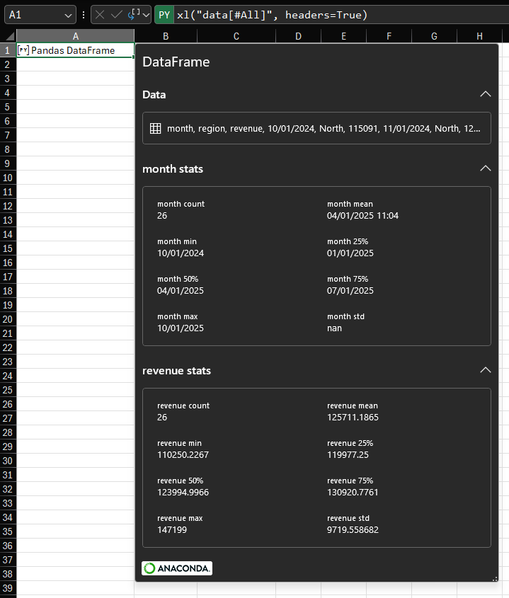
Continuing from last week’s post about custom card views of Python objects, this post will describe how you can override the default card preview of a Pandas DataFrame. By understanding how this is done for one example, you’ll be able to override the default card preview of any Python object in Python in Excel. The default card for a DataFrame This post is using the same data as last week: The default card preview for a DataFrame looks like this: As you can see, we have some information about the number of rows and columns and a preview of the…
-
How to customize card previews for Python in Excel
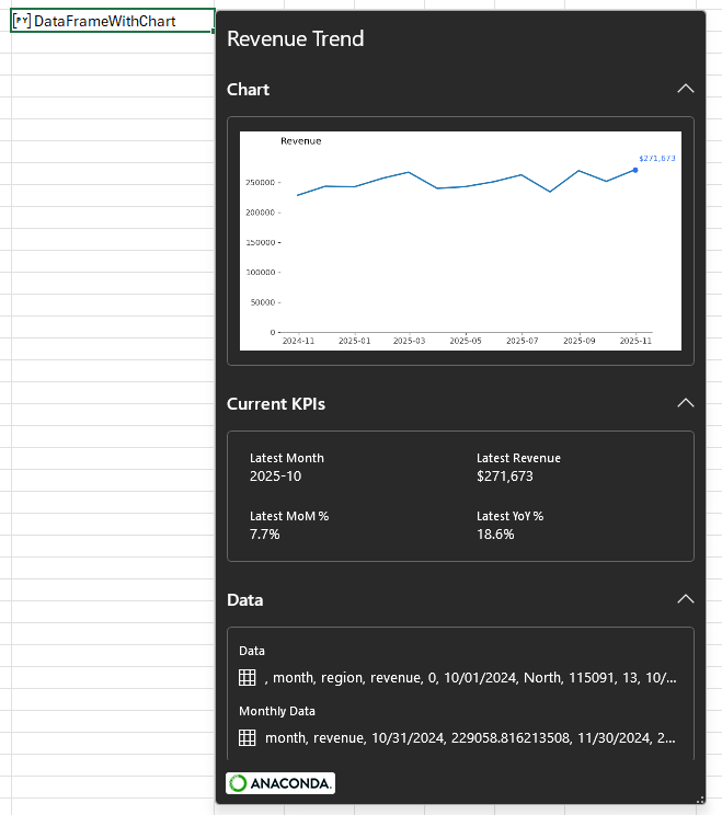
Data The examples in this post will focus on an artificial dataset of revenue by region and month for the 13 months between October 2024 and October 2025. For purposes of demonstration and discussion, there are two regions. Here is a sample: If you want to follow along, use this formula to load the data to your workbook. Paste it as values, then use Ctrl+T to convert it to a Table. Name the Table ‘data’. Introduction To begin with, let’s create a simple Python cell and load the Table ‘data’ into a DataFrame using the xl method: There are two…
-
UPDATE! 🪲 How to make a timestamp column for an Excel Table
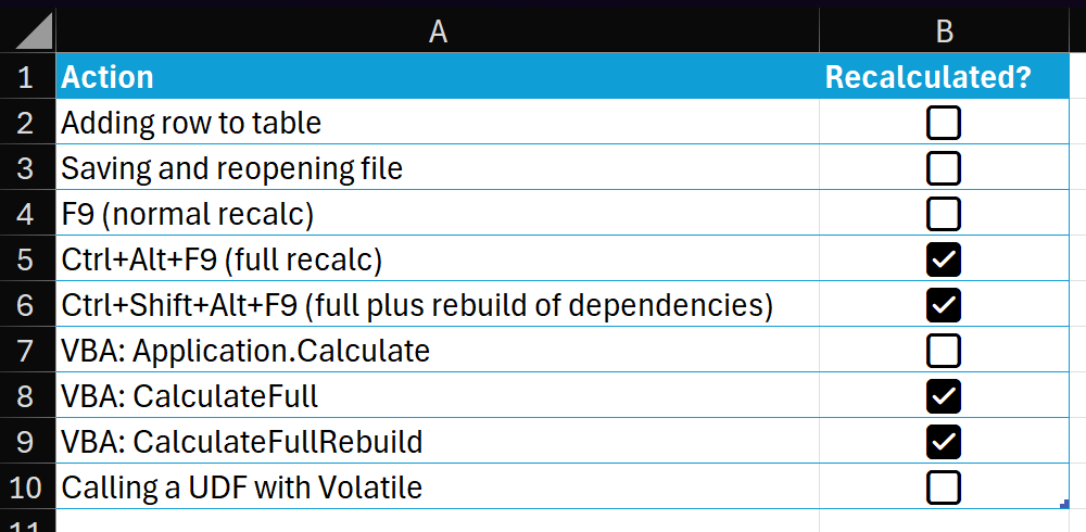
I’m reliably informed by a man on the inside that the capability described below, tantalizing though it may be, is in fact the side effect of a bug! And like many bugs, it will soon be squashed. Flattened. Smooshed out of existence. So be warned! Full credit for the idea in this post goes to Lorimer Miller. I don’t know how he comes across these ideas, but I’m glad he does. Let’s get into it. A reminder about volatility You may have heard about certain Excel functions being volatile. Among them are INDIRECT, OFFSET, NOW, TODAY, RAND and RANDARRAY. There…
-
How to get the current region in Excel with a formula
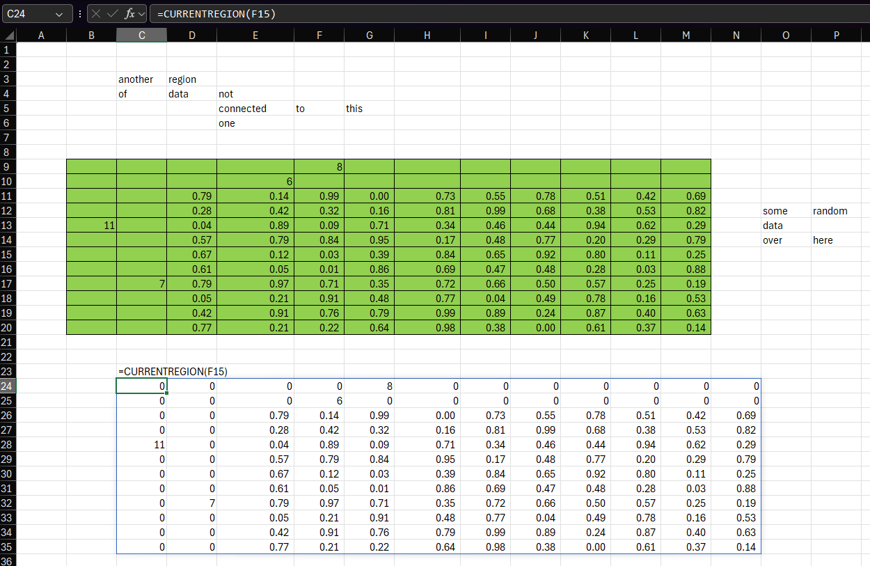
Someone on an email distribution list I’m on said it would be really useful to have a function that mimics the behavior of VBA’s Range.CurrentRegion. I thought this would be an interesting challenge to implement with LAMBDA, so here’s one way you might do it: Here’s an example of the function being used. You can see that the formula in cell C24 is passing F15 to CURRENTREGION, which is then returning the current region from that cell – the equivalent of pressing Ctrl+A. Importantly, it captures the 11 in B13 even though it’s not directly connected to any other data.…
-
How to visualize matrix transformations with Python and matplotlib
Guys. You wouldn’t believe how long it took me to figure out the syntax for correctly displaying a square matrix on a matplotlib plot. And you know why it took so long? Because I tried to get ChatGPT to help me. And it kept. Suggesting. The. Same. Wrong. Answer. Over. And Over. Protip: RTFM. Anyway, here’s a neat Excel workbook with which you can visualize the effect of a matrix-vector dot product. Here’s what it looks like when you use it: You can edit the definition of the vector in E3:E4 and edit the transformation matrix in B3:C4 and the…

-
5 ideas for new SQL features!
Last week I wrote about some of the newer innovations in the SQL space. This got me thinking. What other language features would be useful in a SQL environment? This post explores some ideas I’ve had around this. It’s purely speculative, but perhaps it will spark some ideas for you. 1. Optional GROUP BY clause In most GROUP BY queries, every non-aggregate must be listed in the GROUP BY clause. Sure, we have options, like GROUP BY 1, 2, 3 or GROUP BY ALL, but while these are convenient, they’re also busywork for most queries. So my first suggestion is…

-
SQL is changing into something new – are you ready?
On 30 April 2025, DataBricks announced their SQL pipe operator. Without giving you a full rundown of what it is and what it does, here’s a quick example which should give you a good idea. This query: Is now equivalent to this: There’s more to it of course, but that’s the gist of it. It follows precedent set by other languages. Here’s how it might be written in R using tidyverse syntax. Here’s how you might express it in Python using a method chain. Ok so you get the picture. It’s not an unusual step for DataBricks to have taken.…

-
Exploring NumPy operations with a Python in Excel challenge
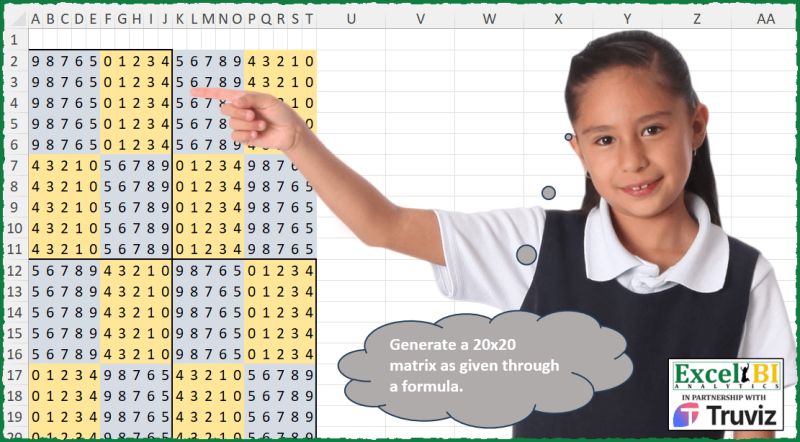
Here’s a data challenge I saw on a LinkedIn post: My goal was to produce the matrix using Python in Excel. The first thing to note is that the matrix is entirely composed of the integers 0 through 9. So: You can see in the image above that the larger matrix is composed of smaller chunks of 5 integers. All of the grey boxes are the integers 5 through 9 either in order or in reverse order. The yellow boxes are the integers 0 through 4, again in order or in reverse order. So we can define two building blocks…
-
Use XLOOKUP and XMATCH with regular expressions (regex)
The Excel team introduced support for regular expressions in May 2024 with three new functions The functions were announced in this post on the Microsoft 365 Insiders blog. As well as these new functions, we learned that we will be able to use regular expressions with XLOOKUP and XMATCH in the near future. Regex coming soon to XLOOKUP and XMATCH We will also be introducing a way to use regex within XLOOKUP and XMATCH, via a new option for their ‘match mode’ arguments. The regex pattern will be supplied as the ‘lookup value’. This will be available for you to…

-
Portfolio – Tableau – Maven Remote Work Challenge
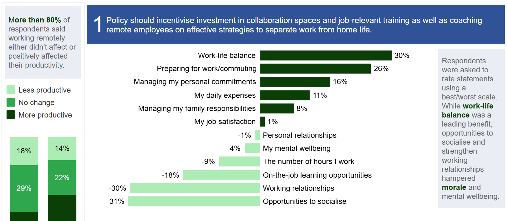
I created this Tableau Report as an entry for the Maven Analytics Remote Work Challenge in March 2022. Click here to view the Jupyter notebook I used to clean the data, which details my thinking and the steps taken.
-
Better regex results with look-behinds
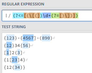
This post will teach you how to write better regex with look-behinds and look-aheads. All the images in this post are from regex101. An example problem Take these text strings for example: Suppose we want to write a regular expression that extracts all numbers of one or more digits that are enclosed by matched brackets. When I say matched brackets, I mean any of these: We can see that the first line has the number 123 within { }, and the number 890 within ( ). The number 4567 is not counted because its opening bracket is { and its…
-
Unfold a list with this new function
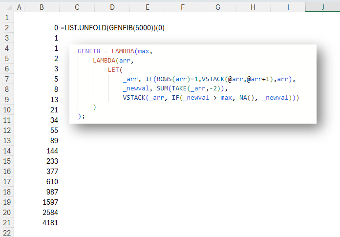
In this post you’ll learn to unfold a list from a value with a recursion wrapper called LIST.UNFOLD. INTRODUCTION In Excel as in many other languages, we can use REDUCE to reduce (or fold) a list into a single value. We iterate over the list, and at each element apply a function. The result of that function becomes what’s known as an accumulator. This accumulator created from applying the function to one element is passed as an argument to the same function when it is applied to the next element. This continues until the last element of the list is…
-
8-Step Process For Writing Recursive Functions in Excel
1. Write a recursive function in Excel2. Realize you could’ve done it with REDUCE3. Write it with REDUCE4. Realize you could’ve done it with dynamic arrays5. Write it with dynamic arrays6. Realize there’s already a built-in function to do it7. Use the built-in function8. 😐

-
Learn A Powerful Technique For Scanning Arrays In Excel
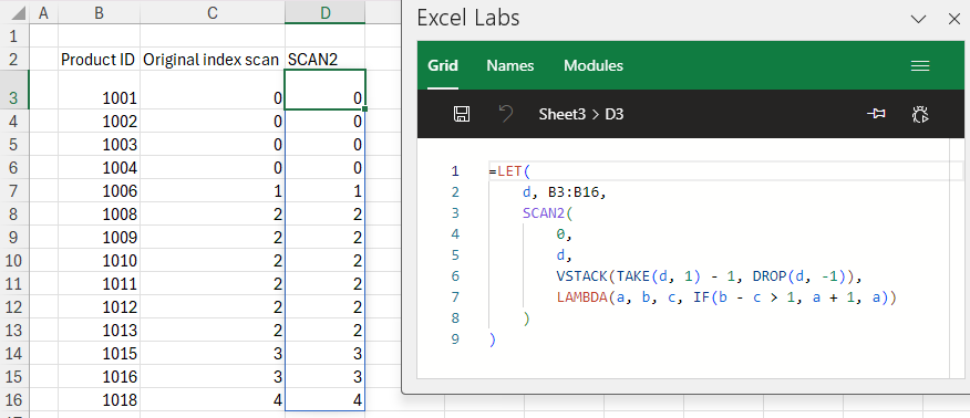
INTRODUCTION In this post, we’ll learn a powerful technique for scanning arrays in Excel. The SCAN and REDUCE functions in Excel allow us to apply a function to each element of an array and, as each function call returns, save the result in an accumulator which is passed as an argument to the function call on the next array element. As a simple example, the following function starts by assigning 0 as the initial value of the accumulator. It then scans over the sequence of integers {1..10} and, for each integer, it adds the current array element to the value…
-
Professional SQL That Will Make Your Queries Shine: INTERSECT vs. INNER JOIN
When working with databases, it’s crucial to know the best methods to query data effectively. In SQL, two powerful operations that allow you to compare sets of data are the INTERSECT operator and the INNER JOIN clause. Both commands serve the purpose of identifying commonalities between datasets, but they do so in subtly different ways that can affect the output and performance of your queries. What is the INTERSECT Operator? The INTERSECT operator is used to return a distinct intersection of two sets, which means it will only return the rows that are present in both query result sets. Here…

-
Free LAMBDA – SUMPRODUCT for 2D arrays
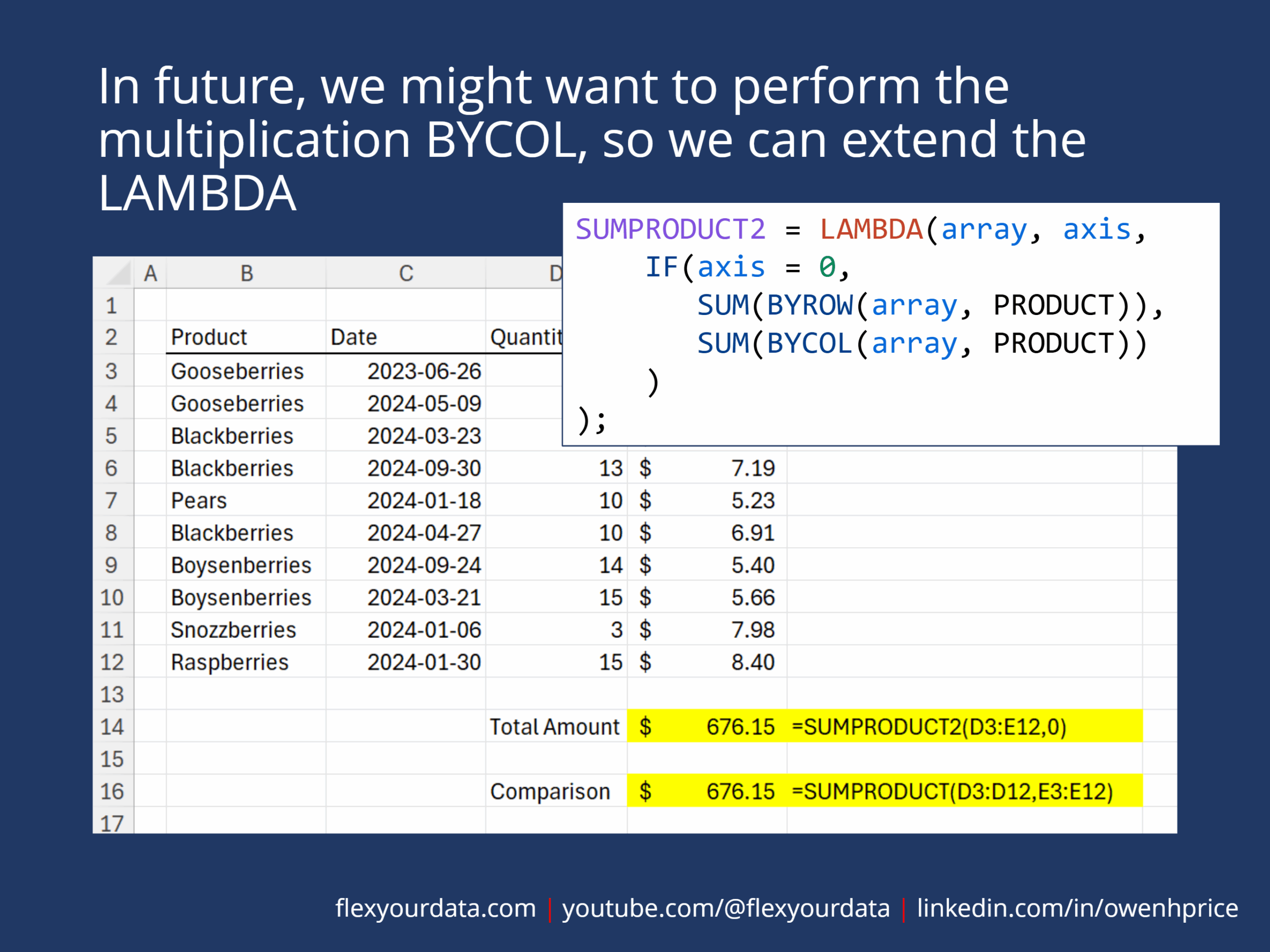
I wanted to be able to pass a 2D array as a single argument to SUMPRODUCT. But it doesn’t work like that, so I worked around it and created SUMPRODUCT2. This document shows my thought process and steps I went through to get to the final result. I hope you find it interesting. Here’s a link to the original post of this content on LinkedIn.
-
Calculate all pairs from two lists in Excel
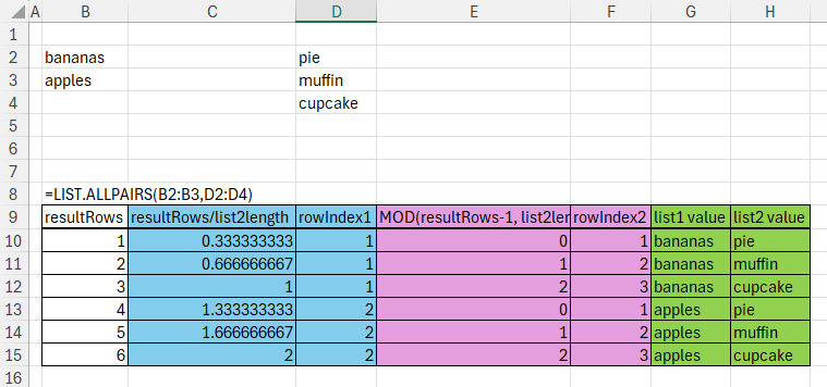
Introduction In this post we’ll look at a way to create a LAMBDA function to calculate all pairs from two lists in Excel. F# has a collection of functions for working with lists. Without getting into the details of F# itself, a list is a collection of items. It’s quite similar to a list in Power Query’s M language. In fact, M is so similar because it is partly based on F#. One of the functions which can be used for manipulating and working with lists in F# is called List.allPairs. This function accepts two lists. In Excel terms, let’s equate…
-
The SWITCH and LET functions – Excel formula performance
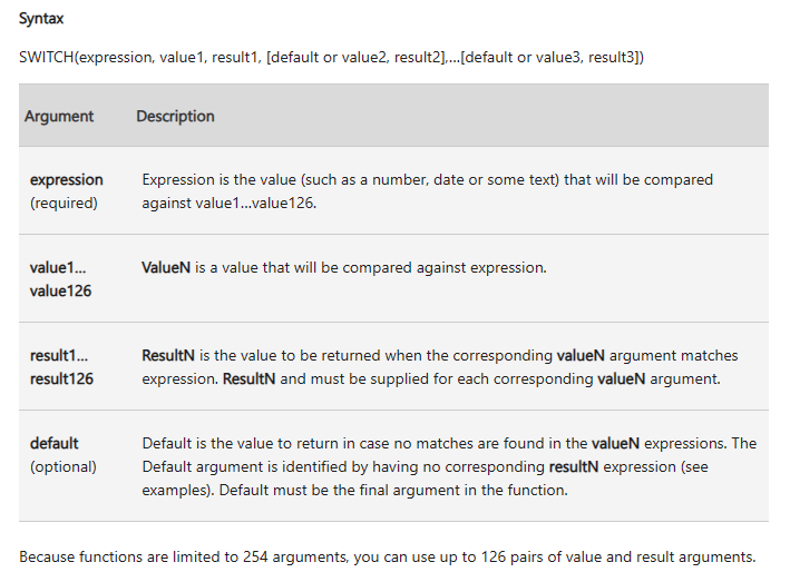
Let me get right to the point. Both SWITCH and unused complex names in LET can slow down your formulas Introduction This formula returns a large array: In the Beta version of Excel I’m using, the above formula can be written like this: I’ll use the shorter version for the remainder of this post. This MAKEARRAY formula creates an array of 10000 rows and 1000 columns. For each cell in the array, it uses the PRODUCT function to multiply the row number by the column number. It takes my computer about 3 seconds to return this formula. By most measures,…
-
Excel LAMBDA: simplified rolling aggregate of any function
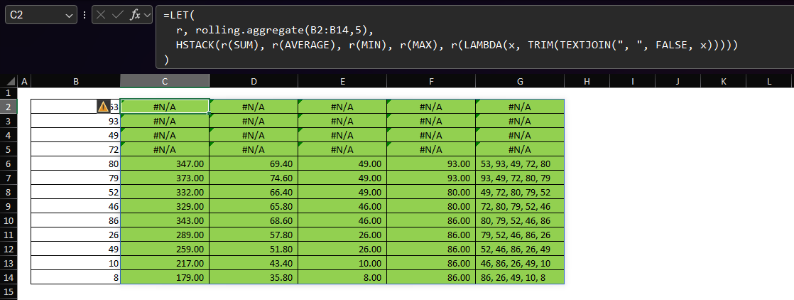
The gist for this lambda function can be found here. Preface This post is a follow up to an earlier post. I wrote the function described there in May of 2022, before I had access to functions like VSTACK and HSTACK and before I had a solid understanding of SCAN and REDUCE. As such, while it was fun to write and worked just fine, it was a monster of a function! The recent release of the GROUPBY and PIVOTBY functions (described here) also came with a huge upgrade to the LAMBDA experience. To cut a long-story short, with this release,…
-
Breadth-first search using Excel
The code shown in this post can be found here. What is breadth-first search? Breadth-first search is a popular graph traversal algorithm. It can be used to find the shortest route between two nodes, or vertices, in a graph. For a good primer on how this algorithm works, you can watch this video: Put simply, breadth-first search, which for the remainder of this post I’ll refer to as BFS, uses a queue data structure to prioritize which nodes of the graph to visit next. The important thing to remember about a queue is that it is a first-in-first-out data structure…

-
Excel LAMBDA: Create a list of integers
The gist for this lambda function can be found here. The goal Sometimes we may want to create a simple list of integers from some starting value to some ending value. This is easy enough with the SEQUENCE function. For example, suppose we want to create a list of integers from 1 to 10. This is really all it takes: The first parameter is the number of rows we want in the sequence. The remaining parameters default to 1, so the formula above is equivalent to this: Above, the second parameter is the number of columns we want, the third…

-
Excel LAMBDA: parameter checks and function validation
It turns out that if we pass an Excel lambda function as a parameter to another Excel lambda function, we can’t then test that the function passed into that parameter is from a list of allowed functions. Calling the wrapper lambda with any of the other three functions defined below as its sole parameter will cause a #VALUE! error. This is because we can’t use a lambda in the SWITCH function in this way and we can’t use a lambda as an operand with the equals operator. Because of this, if we want to validate which function was passed as…
-
excel-lambda-ROTATE: rotate an array in Excel
The lambda described in this post is in the LAMB namespace, the gist for which can be found here. The goal TRANSPOSE is great. But sometimes it doesn’t do everything I’d like. So, the goal here is: Create a lambda function that will rotate an array by 90 degrees an arbitrary number of times A solution Here’s a function I’ve added to the LAMB namespace which I call ROTATE: ROTATE takes these parameters: arr – an array you want to rotate times – a non-negative integer representing the number of times you want to rotate the array anti-clockwise by 90…
-
Excel LAMBDA: outlier detection functions
The gist for this namespace can be found here. You can download a workbook containing the sample data (sulphates column from Kaggle wine quality dataset), the LAMB namespace, and the OUTLIER namespace here. The goals This is the second of a two-part blog post covering some work I’ve been doing to update and improve some functions to assist with outlier detection. Both posts are a follow-up to a post I wrote in April 2022. If you’d like to read some of the reasoning and background as to why we would bother creating functions for outlier detection, please read that post first.…
-
Excel LAMBDA: Introducing the LAMB namespace
The gist for this namespace can be found here. The goals When I was first learning about LAMBDA in Excel, I wrote some functions to calculate outlier tests against a column of data. The main function – OUTLIER.TESTS – allowed us to write a single formula, apply a collection of transformations, and run a standard deviation test against each of the transformations of the variable. It was really exciting to me that we could now do this so easily in Excel. You can see how it works below. Each test returns three columns indicating which rows in the transformed data…
-
How and why to use namespaces for Excel Lambda functions
In programming, a namespace is a grouping for procedures, methods, objects and other code that are related to each other. We can store Excel Lambda functions in namespaces to keep them organized. The Advanced Formula Environment To create a namespace, you will need the Advanced Formula Environment (AFE). If you don’t have AFE, you can download and install the free add-in here. Creating a namespace There are two ways to create a Lambda namespace in Excel. 1: From scratch Open AFE. If you haven’t changed your ribbon, after you install AFE it will be on the far right-hand side of…
-
Video – Learn how to use functions as parameters in Excel
An important concept in functional programming is that of functions as parameters. With the introduction of the LAMBDA function, this is now possible in Excel. This short video briefly introduces this concept.
-
Video – Detailed walkthrough of creating a Depreciation Schedule LAMBDA function
This post is a follow-up to the original excel-lambda-depn.schedule post. I created the video below to show the steps involved in creating that LAMBDA from scratch, including a modification which allows the schedule to be produced by month as well as by year. some of the text in the video is quite small, so I recommend a resolution of no lower than 480p (higher if possible) and full screen. Chapter links are available in the video description on YouTube.
-
Create a depreciation schedule in Excel with one function
The gist for the lambdas shown in this post can be found here. When importing this gist, be sure to select “Add formulas to new namespace” and use the name “depn”. The goal There are several methods of calculating depreciation in Excel. The functions SLN (straight line) , DB (declining balance) , DDB (double declining balance) and SYD (sum-of-years’ digits) are commonly used. In addition, it’s useful to calculate a table showing the depreciation in each period over the life of the asset. As an example, this table shows the depreciation of an asset with a life of 9 years using…
-
Lambda presentation to Microsoft Excel and Data Analysis Learning Community on July 31st, 2022
On July 31st, 2022, I gave a presentation about Excel Lambda functions to the MS Excel Toronto Meetup group. If you have any questions about the content of the video or the file, please leave a comment.
-
Classify data using K-nearest neighbors (KNN) in Excel
The gist for this lambda function can be found here. The goal The goal in this post is: Create a function to classify data using K-nearest neighbors (KNN) in Excel A solution Here’s a lambda function called KNN: I’ve also included the definition of the FREQ.SIMPLE lambda function. That function produces a two-column frequency table of counts of unique values in a column of data. For details of how that function works, you can read this post. KNN has three parameters and as such accepts three arguments. x – an observation (row) in need of classification. This is an array…
-
Create a simple frequency table in Excel with one function
The gist for this lambda function can be found here. The goal The goal in this post is: Create a simple frequency table in Excel with one function A solution Here’s a lambda function called FREQ.SIMPLE: FREQ.SIMPLE has one parameter and as such accepts one argument. data – a single-column array of data. This is usually a column of text values with some duplication and we want to count the occurrences of each unique value in the column. How it works Here’s how it works: This is a very simple function, written initially to be used by other functions, such…
-
Lambda presentation to MS Excel Toronto Meetup Group on July 13, 2022
On July 13th 2022, I gave a presentation about Excel Lambda functions to the MS Excel Toronto Meetup group. You can download the file used in the presentation here. If you have any questions about the content of the video or the file, please leave a comment.
-
Convert recipe ingredients to different units in Excel
The gist for this lambda function can be found here. The goal Here’s a picture of a red velvet cake I baked last week. I baked this cake from scratch for my son’s birthday. I’m not a baker. But it makes a nice change from working with computers. Because I’m English, I get most of my recipes from BBC Good Food. The recipe I used is here. I live in the US. This means most of my ingredients have the wrong units of measure which don’t necessarily fit with recipes published by the BBC and my measuring instruments are wrong…
-
Calculate holiday dates for any year in Excel
The gist for this lambda function can be found here. You can download a workbook with example definitions of relative and fixed holidays here. The goal When working with dates in Excel, it’s sometimes useful to have an accurate list of the public holidays in a given year so we can calculate (for example) the working days between two dates. We might also want to create a simple attendance calendar and need to know which dates should be excluded. So, the goal here is: Create a lambda function that will return a list of holidays for an arbitrary year based…
-
Calculate effective interest rate in Excel without iterative calculation
The gist for this lambda can be found here. The goal I saw a video from Diarmuid Early in which he discusses the use of the iterative calculation setting in Excel for calculating effective interest rates. I share a similar view that using that setting can be very dangerous and if possible, it’s best to avoid it. So: Create a simple recursive lambda function that can be used to converge on an effective interest rate (i.e. that includes “interest on the interest”) I’d like to preface this post by saying that the lambda shown here is based on a very…
-
Create a list of dates for a payment schedule in Excel
The gist for this lambda function can be found here. The goal Inspired by Diarmuid Early‘s YT video “Debt 101” and Brent Allen‘s “Generating an Amortization Schedule” post on his blog, the goal here is Simplify the creation of a series of dates to be used as payment dates for a debt instrument This series of dates should: start on or before the start date of the debt finish at the end of or after the end of the term of the debt separate each date by a parameterized number of months (the period) A solution Here’s a lambda function…
-
What’s the difference between ROLLUP and GROUPING SETS in SQL?
The full script for this post can be found here. This post uses the AdventureWorksDW database in SQL Server 2019 Express. Depending on your preference, you can either watch this video or read below. The goal Suppose we have a request to produce a report: Create a report showing internet sales amount with these columns: Order year Country Product category Sales amount Include a sub-total row showing total sales amount for each year. The value in the Country column on the sub-total row should be “All countries in YYYY”. The value in the Product category column on the sub-total row…
-
Excel – Introduction to Analyze Data (video)
Watch the video below and learn about Analyze Data in Excel. The limitations of Analyze Data and why it sometimes won’t work Use Natural language to Automatically discover insights in your data Automatically create useful pivot tables and pivot charts Automatically recognize mis-spelled column names Automatically filter your data without writing complex functions
-
Calculate a correlation coefficient matrix in Excel
The gist for this lambda function can be found here. The goal When we have a dataset with lots of variables (features), we can simplify the modeling process by first trying to determine which variables are correlated with one another. If two variables are highly correlated, we can consider including only one of them in the model we build. Excel provides a feature in Data Analysis Toolpak called “Correlation”. This function can be accessed by enabling the Data Analysis Toolpak, then following the on-screen instructions for the Correlation function. The output of this feature is to produce the lower-triangular correlation…
-
SQL: Numerical row constructor comparisons in PostgreSQL and MySQL
The full script for this post can be downloaded here. The following post was written primarily in Postgres 14 and tested in both Postgres and MySQL. While the data generation and use of EXCEPT are not supported natively in MySQL, the principles of row comparisons are equivalent. Setup To demonstrate how a row constructor comparison can be confusing, let’s create some dummy data with two columns of integers: Comparisons PostgreSQL allows us to compare two sets of values using what is known as a row constructor comparison. A row can be constructed with parentheses, like this: We can create…
-
SQL: Use LAG and SUM window functions to group rows
What is Advanced SQL, anyway? I think about this sometimes. Is it window functions? CTEs? I don’t know. Some of it is trickier than others. I think it’s relative to how much practice you’ve had and depends a great deal on the data in front of you. Anyway, I saw this post on LinkedIn by Ankit Bansal. It struck me as an interesting problem. I wanted to come up with a solution before watching the author’s video. It’s only 8 minutes, so probably worth watching. I was happy to find that my solution was close but not identical. In case…
-
An Excel lambda function for DENSE_RANK from SQL
The gist for this lambda can be found here. The goal There are many reasons for ranking data. Excel provides a few native functions to do so. The two main ones are RANK.AVG and RANK.EQ. Each function will return the integer rank of a number within a list of numbers, sorted either descending or ascending order. To understand how each function works, take a look at this simple example: You can see that when RANK.AVG encounters two identical numbers (the population in millions of Iran and Turkey), it takes the two ranks they would otherwise receive – 17 and 18…
-
Calculate rolling sum in Excel (and much more)
The gist for this lambda function can be found here. You can download an example file here. The goal If we have a table of sales of a product where each row represents one month, then we might want to calculate – for each month – the rolling sum of sales over the most recent three months. When we sum a variable over multiple rows like this, the rows we are summing over are referred to as a “window” on the data. So, functions that apply calculations over a rolling number of rows are referred to as “window functions”. These…
-
What is a thunk in an Excel lambda function?
This is my attempt to answer a question I have asked myself many times over the last few months: What is a thunk in an Excel lambda function? Background Many of the new dynamic array functions that create arrays, such as MAKEARRAY, SCAN, REDUCE and so on, will not allow an element of the array created to contain an array. In short, an array of arrays is not currently supported. As an example, consider the SCAN function. The description on the support site says Scans an array by applying a LAMBDA to each value and returns an array that has…
-
Group a continuous variable into bins of equal counts
The gist for this lambda function can be found here. The goal It’s sometimes useful to be able to group a continuous variable into bins of equal counts such that we can work with that variable as it if were discrete. In mathematics and machine learning applications, this process is sometimes referred to as “discretization”. If you’re an Excel user or statistician, you may know it as “binning”. In short, we want to assign a group to each value in an array, such that the count of values in each group is equal, or as close to equal as possible.…
-
Convert currency stored as B or M to a number with just one function
The gist for this lambda function can be found here. The goal Sometimes we might have numbers in an Excel file formatted like this: I’d like to create a function that those values into a number where each value is at the same scale. A solution I say “a” solution, because I’m sure there are many others. Here’s a lambda function called CLEANCURRENCYTEXT: CLEANCURRENCYTEXT takes two arguments: val – this is the value which is currently stored as text and usually has a suffix at the end indicating it’s billions, or millions, or similar [mapping] – this is an optional…
-
Convert currency stored as B or M to a number in PowerQuery
The gist for this pattern can be found here. The goal Sometimes we might have numbers in a text file formatted like this: I’d like to create a custom column that converts this text into a currency data type, preserving the scale of the suffix in each row and preserving the currency symbol. A solution I say “a” solution, because I’m sure there are many others. Here’s a snippet we can paste into the Advanced Editor. Alternatively, we can just paste lines 2 through 41 into a Custom Column dialog. I know, it looks long, but I’ve put a lot…
-
Transform, test and flag a variable for outliers in Excel with one function
The gist for this set of functions can be found here. The goal This post is not intended to be an instruction on the mathematics or theory of outlier detection. My intention is to demonstrate another way we can use lambda in Excel to simplify a common task. This post will show you how to create a lambda function that will: Transform a continuous variable to correct for right-skew Calculate the upper and lower boundaries outside which we might consider a data point to be an outlier Return a dynamic array that includes The original data The transformed data A…
-
Build a forecast for comparison with actuals with a single formula
The gist for this lambda function can be found here. Forecasting in Excel Excel comes with several functions that allow us to quickly produce forecasts on time-series datasets. Data>Forecast Sheet One method you can use is the “Forecast sheet” button which can be found on the “Data” tab of the ribbon in Excel versions 2016 onwards. For a primer on what that does and how it works, I encourage you to watch this video. The “Forecast sheet” button uses the FORECAST.ETS function to produce a table where the original values are in one column and the forecast values are in…
-
Calculate % growth of current month over 12 months before
The gist for this lambda function can be found here. I was straining my brain to understand the lambdas posted by user XLambda on the lambda forum at mrexcel.com. This person is really mining the depths of what’s possible with lambda in Excel. I go there frequently when I want to understand how to do something. While reading about ASCAN, I found myself watching this video by Leila Gharani which showed how to calculate year-to-date sums (YTD) using the SCAN function. This got me thinking about a common calculation I’ve seen used in my work over the years Calculate the…
-
UPDATED AND IMPROVED – Get descriptive statistics in Excel with just one formula
Quick start If you want to use this function to get descriptive statistics in Excel with just one formula and without reading all the detail below, you will need to: create a LAMBDA function called RECURSIVEFILTER using this gist create a LAMBDA function called GROUPAGGREGATE using this gist create a LAMBDA function called DESCRIBE using this gist If you’re not sure how to create a LAMBDA function, read “Step 3 Add the Lambda to the Name Manager” under “Create a Lambda Function” on this page. The DESCRIBE LAMBDA function This post is a follow-up to an earlier post about an…
-
Calculate the Levenshtein Distance in Excel
The gist for this lambda function can be found here. A friend of mine challenged me to implement a LAMBDA to calculate the Levenshtein Distance in Excel. As a reminder, the Levenshtein Distance represents the fewest number of insertions, replacements or deletions that are necessary to change one text string into another. For example, given the words “kitten” and “sitting”, we need these operations to change the former to the latter: Replace the k with an s Replace the e with an i Insert a g at the end We can think of this as a measurement of similarity between…
-
Quickly create summary tables in Excel with just one formula
The gist for this lambda function can be found here. Let me cut to the chase. I have some data from Wikipedia for population by country . I’ve also got some data of land area by country, from here. I created a Power Query to merge them. The output looks like this: There are 195 rows in this table. I would like to create a summary table with these columns: Region Comma-separated list of countries in the region Total population of the region Maximum land area of any country in the region The requirement to have a comma-separated list means…
-
Use Excel’s FILTER function with dynamic lists of filters
The gist for this lambda function can be found here. Excel’s FILTER function lets you take an array of data (or a table, or a range) and filter it with an “include” array of TRUE/FALSE values, where each row in the include array corresponds to each row in the data array. If the include array is TRUE, FILTER returns that row from the data array. If it’s FALSE, it doesn’t. Here’s an example of how it works. Suppose we have some data from Wikipedia about the populations of various countries. We can use FILTER to filter the table for just…
-
Get descriptive statistics in Excel with this LAMBDA function
The lambda described in this post has been updated with additional features. You can read that post here. You can use the Data Analysis Toolpak to get descriptive statistics in Excel for a variable in your data. First, you need to make sure the analysis toolpak is activated as an Add-in: Then you select “Data Analysis” from the Data tab on the Ribbon, and do this: These statistics can be useful in situations where you’re looking at your data for the first time and want to get a general feel for its shape and characteristics. To shortcut this exercise, I…
-
One-hot encode categorical data with LAMBDA
The gist for this lambda function can be found here. One-hot encoding. Create as many columns as there are unique values in a variable. Put a 1 in a cell if the column and row represent the same value, otherwise put a zero in the cell. Use these new columns to create ML models. Do it in Python. Do it in R. Do it in Excel, if the mood takes you. That’s right. You can one-hot encode categorical data in Excel. Use this: Let’s break it down: ONEHOT has one argument: a single-column range of data that includes a column…
-
Get n-grams from a text string using this LAMBDA function
The gist for this lambda function can be found here. A common task in Natural Language Processing (NLP) is to tokenize text strings into n-grams. This can be done easily in languages like Python, Scala, R and others. They have very good libraries for performing that kind of task at scale. I wanted to see whether something like that would be possible with an Excel LAMBDA function. I call this NGRAMS and at the moment, it splits text into arrays of words of n words each. It takes three arguments: text – the text you want to calculate n-grams for…
-
Excel: Un-Merge Cells And Fill Each Cell With Original Value Using VBA
Do you sometimes receive a file with merged cells all over the place? Something like this: The first thing I want to do in that situation is un-merge everything. Well, that’s easy enough. If I use the Merged Cells button on the ribbon, it will do this: Ok, now I need to fill in the blank rows with the category header from the top of each row. I can do that using the useful technique of Go To Special/Blanks and enter a formula. Like this: That is useful, but I don’t particularly like having formulas in those cells after I’m…
-
Format A Row Of Data For SQL INSERT
The gist for this lambda function can be found here. If you sometimes need to quickly put some Excel data into a SQL table or use the data in a CTE, you may have found yourself doing something like this: Here’s a LAMBDA I’ve called SQLVALUES: =LAMBDA(t,LET(d,IFS(ISTEXT(t),”‘”&SUBSTITUTE(t,”‘”,”””)&”‘”,ISBLANK(t),”NULL”,LEFT(MAP(t,LAMBDA(x,CELL(“format”,x))),1)=”D”,TEXT(t,”‘YYYY-MM-DD HH:mm:ss’”),TRUE,t),”(“&TEXTJOIN(“,”,FALSE,d)&”)”)) This will: Wrap the tuple in parentheses Wrap text and dates in single-quotes Replace embedded single-quotes with escaped single-quotes Separate the columns with commas Format date-formatted cells as YYYY-MM-DD HH:mm:ss If we’re inserting multiple values and our SQL database supports a list of tuples, we can also do this: =LET(arr,A2:C6,BYROW(arr,SQLVALUES)&IF(LASTROW(arr),”;”,”,”)) Which is…
-
Split An Alphanumeric String Into An Array Of Characters
=LAMBDA(rng,vertical,LET(chars,MID(rng,SEQUENCE(LEN(rng)),1),IF(vertical,chars,TRANSPOSE(chars)))) This LAMBDA function takes two arguments: rng – a cell containing a text string vertical – TRUE/FALSE. If TRUE, the LAMBDA will return a vertical array of the characters in rng. If FALSE, the LAMBDA will return a horizontal array of the characters in rng In my file, I have named this LAMBDA “CHARACTERS”. You can of course call it whatever you want. So what? This is useful, because it simplifies things when we want to extract all the numbers or text from a character string. To get all the numbers in a horizontal array: =LET(c,CHARACTERS($A$1,FALSE),nums,INT(c),FILTER(nums,NOT(ISERR(nums)))) To…
-
Filter Out Rows With Empty Cells
If you want to quickly get all rows which don’t have any blanks in any columns, you can combine FILTER, BYROW and AND, like this: =FILTER(range,BYROW(range,LAMBDA(r,AND(r<>””)))) Here, I’ve defined a LAMBDA function, which is really just a way of applying some logic (in the second parameter) to some data (in the first parameter). I have “r” as the name for my data. By passing that LAMBDA as the second parameter of BYROW, I’m telling Excel that “r” represents a row of “range” and that I want the function AND(r <> “”) to be applied to that row. That AND function…
-
Excel: Calculate The Difference Between “Percentage Of Column Total” Columns
I downloaded some data from the USDA FAS custom query builder. The file contains the area harvested of corn in many harvest years for non-US countries. I want to calculate the % of non-US corn area that each country represents in the latest two full harvest years and then calculate the change in percentage points between those two years. The downloaded data looks like this: I’m going to use the harvest years “2017/2018” and “2018/2019”. The first thing I’ve done is format the data as a table, by selecting anywhere in the data and pressing Ctrl+T, then I’ve given the…
-
Excel: Use Names To Make Your Formulas Easier To Read
There’s a useful but under-used feature in Excel that can make your formulas much easier to read and understand. In the image below, the Name Box is the white box where it says A2. You can see that I have an Important Value in cell A2. I’m going to use that value all over my workbook in lots of formulas. If I want my formulas to be easier to read, I can give cell A2 a name by typing something in the name box. I’ve given cell A2 the name “importantvalue”. Now I can use that name in my…