Breadth-first search using Excel

The code shown in this post can be found here.

What is breadth-first search?

Breadth-first search is a popular graph traversal algorithm. It can be used to find the shortest route between two nodes, or vertices, in a graph.

For a good primer on how this algorithm works, you can watch this video:

Put simply, breadth-first search, which for the remainder of this post I’ll refer to as BFS, uses a queue data structure to prioritize which nodes of the graph to visit next. The important thing to remember about a queue is that it is a first-in-first-out data structure (FIFO), which means that items added to the queue earlier are removed from the queue in the order they’re added. 

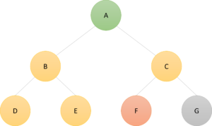
Consider this graph where we want to find the shortest route from node A to node F:

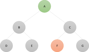
We can represent this graph in Excel in several ways. Here’s one, which shows each node and the neighbors of that node:

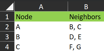
BFS starts by adding node A to the queue.

Queue = {A}

We also initialize a secondary data structure, typically a dictionary or in Excel terms, an array, that keeps track of the nodes we have already visited along with where they were visited from. Because A was the start, we initialize it as follows:

Visited = {A: None}

The algorithm continues as follows:

First iteration

1. Dequeue an item from the queue.

This removes the left-most (first-in) node from the queue and makes it the current node. On the first iteration, this is just Node A. So:

Current node = A

2. Is the current node the goal?

If A = F, then exit the algorithm. Otherwise:

3. For each node adjacent to the current node

i.e., the yellow nodes B and C

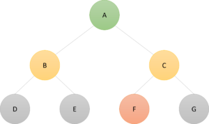
Is the node under consideration in the visited array? If not: (a) add it to the queue and (b) add it to the visited array.

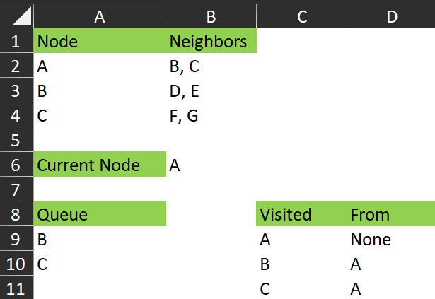
After the iteration, we have:

Queue = { B, C }

(because B was added to the queue, then C was added to the queue)

Visited = {A: None , B: A, C: A}

(because B and C were visited from A, in that order)

Represented in Excel, the state of the data at the end of the first iteration:

Second iteration

1. Dequeue an item from the queue.

This removes the left-most (first-in) node from the queue and makes it the current node. The left-most item in the queue is B, so:

Current node = B

2. Is the current node the goal?

If B = F, then exit the algorithm. Otherwise:

3. For each node adjacent to the current node

i.e., the yellow nodes D and E

Is the node under consideration in the visited array? If not: (a) add it to the queue and (b) add it to the visited array.

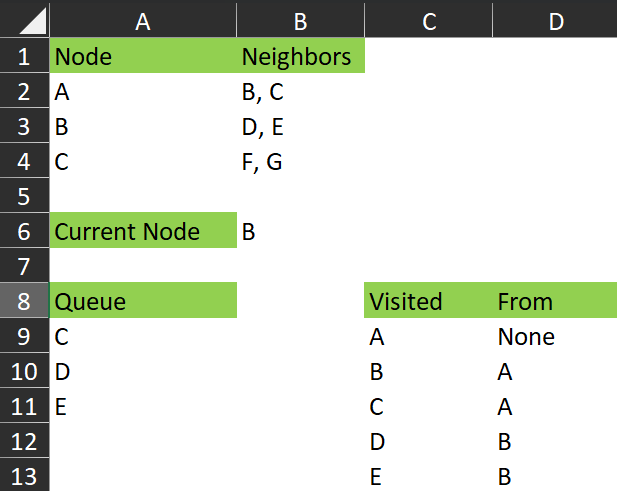
After the iteration, we have:

Queue = { C , D, E }

(because D was added to the queue, then E was added to the queue)

Visited = {A: None , B: A, C: A, D: B, E: B }

(because D and E were visited from B, in that order)

And in Excel, we have this:

And so on

The algorithm continues in in this way, successively adding items that haven’t yet been visited to the end of the queue and removing one item at a time from the front of the queue and checking if it’s the goal.

In the end, the visited array from this example looks like this:

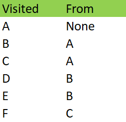
At this point, the algorithm encounters node F and exits because it’s reached the goal. From this visited array, we can see that F was reached from C and C was reached from A, making the path from A to F:

A – C – F

Let’s see how we can automate this process with a lambda function or two.

The goal

Create lambda functions that will calculate a breadth-first search and return various artifacts to help with analysis of paths between nodes of a graph.

A solution

graph.breadth_first_search

All of the following functions I am using in a namespace called “graph”. 

breadth_first_search = LAMBDA(queue, end, [visited], [iteration],
    LET(
        _iteration, IFOMITTED(iteration, 1, iteration + 1),
        _node, INDEX(TAKE(queue, 1), 1, 1),
        _visited, IFOMITTED(visited, HSTACK(_node, "None")),
        _is_undiscovered, LAMBDA(node, ISERROR(XMATCH(node, TAKE(_visited, , 1)))),
        _neighbors, graph.get_neighbors(_node),
        _end_is_neighbor, NOT(ISERROR(XMATCH(end, _neighbors))),
        _newqueue, 
        IF(
            OR(ISERROR(DROP(queue, 1))),
            _neighbors,
            REDUCE(
                DROP(queue, 1),
                _neighbors,
                LAMBDA(a, b, IF(_is_undiscovered(b), VSTACK(a, b), a))
            )
        ),
        
        _newvisited, REDUCE(
            _visited,
            _neighbors,
            LAMBDA(a, b, IF(_is_undiscovered(b), VSTACK(a, HSTACK(b, _node)), a))
        ),
        _result, IF(
            OR(_node = end, _end_is_neighbor),
            VSTACK(_visited, HSTACK(end, _node)),
            graph.breadth_first_search(_newqueue, end, _newvisited, _iteration)
        ),
        _result
    )
);

graph.breadth_first_search takes two required parameters:

1. queue – which is the state of the queue object during the iteration being passed to the function (this function is recursive). When called from the spreadsheet, the queue parameter is passed the “from” node – i.e. the start of the search. This is consistent with the initialization of the search as described above, where the start node is placed in the queue when the algorithm begins. 
2. end – the goal node (i.e. the node we are searching for).

And two optional parameters, which are used by the recursion and generally do not need to be passed to the function when calling it from a spreadsheet:

1. [visited] – this is the current state of the visited array as described above. As the function iterates/searches, more and more nodes are added to the visited array. 
2. [iteration] – this is a simple integer counter which keeps track of how many iterations have been used. I used it to help with debugging while writing the function.

The function defines names using LET:

• _iteration – here we provide a default value of 1 for the optional [iteration] parameter, otherwise if [iteration] is passed to the function, we increment it by one, indicating that we have passed into a new iteration
• _node – since BFS is a FIFO (first-in, first-out) function, we use TAKE(queue, 1) to take the first item from the queue. Since TAKE returns an array, and we need _node to be a single value and not a single-cell array, we use INDEX(arr,1,1) to convert it. _node is then the “current node” as described above. 
• _visited – here we are using a helper function I’ve called IFOMITTED, which replaces the oft-used pattern IF(ISOMITTED([optional parameter]),”some default”,[optional parameter])). So, here if the [visited] parameter is omitted from the function call, the default is to initialize it with HSTACK(_node, “None”), which is consistent with the explanation given above. As a side note, I’ve made a request to have a function called IFOMITTED added to Excel. I would really appreciate if you could go to the page and vote for the idea. The page is here. For now, the IFOMITTED function I’m using in this example is defined like this:

IFOMITTED = LAMBDA(arg, then, [else],
    LET(_else, IF(ISOMITTED(else), arg, else), IF(ISOMITTED(arg), then, _else))
);

• _is_undiscovered – this embedded LAMBDA function checks if a node passed to it already exists in the first column of the _visited array. If it does not exist in that column, this function returns TRUE. 
• _neighbors – here we use a function called graph.get_neighbors to retrieve the nodes connected to the current node. I’ll first explain how that works before continuing with this explanation of graph.breadth_first_search.

graph.get_neighbors

data = Sheet1!A2:B4;

get_neighbors_fn = LAMBDA(data,
    LAMBDA(node,
        LET(
            _neighbors, INDEX(FILTER(TAKE(data, , -1), TAKE(data, , 1) = node), 1, 1),
            TEXTSPLIT(_neighbors, , ", ")
        )
    )
);

get_neighbors = graph.get_neighbors_fn(graph.data);

You can see that the get_neighbors function is calling graph.get_neighbors_fn(graph.data).

graph.data is a named range pointing to the data in the workbook that contains the graph definition.

When we pass the data to graph.get_neighbors_fn, it returns the inner function:

    LAMBDA(node,
        LET(
            _neighbors, INDEX(FILTER(TAKE(data, , -1), TAKE(data, , 1) = node), 1, 1),
            TEXTSPLIT(_neighbors, , ", ")
        )
    )

This inner function assumes the data are formatted as in the example above – two columns with the node in the first column and the neighbors of that node in the second column.

It filters the data to find the node passed to its parameter, returning the cell containing the neighbors of that node, then splits the comma-separated neighbors into an array.

The array of neighbors is then returned to the calling function.

The reason I separated this “get neighbors” process into a different function was so that the breadth_first_search function could be used with other functions to return the neighbors of a given node, which may then be defined on graph data structured in a different way to this example. 

Anyway, let’s continue looking at breadth-first search.

graph.breadth_first_search (continued)

As a reminder, here’s the code again:

breadth_first_search = LAMBDA(queue, end, [visited], [iteration],
    LET(
        _iteration, IFOMITTED(iteration, 1, iteration + 1),
        _node, INDEX(TAKE(queue, 1), 1, 1),
        _visited, IFOMITTED(visited, HSTACK(_node, "None")),
        _is_undiscovered, LAMBDA(node, ISERROR(XMATCH(node, TAKE(_visited, , 1)))),
        _neighbors, graph.get_neighbors(_node),
        _end_is_neighbor, NOT(ISERROR(XMATCH(end, _neighbors))),
        _newqueue, 
        IF(
            OR(ISERROR(DROP(queue, 1))),
            _neighbors,
            REDUCE(
                DROP(queue, 1),
                _neighbors,
                LAMBDA(a, b, IF(_is_undiscovered(b), VSTACK(a, b), a))
            )
        ),
        
        _newvisited, REDUCE(
            _visited,
            _neighbors,
            LAMBDA(a, b, IF(_is_undiscovered(b), VSTACK(a, HSTACK(b, _node)), a))
        ),
        _result, IF(
            OR(_node = end, _end_is_neighbor),
            VSTACK(_visited, HSTACK(end, _node)),
            graph.breadth_first_search(_newqueue, end, _newvisited, _iteration)
        ),
        _result
    )
);

Continuing where we left off:

• _end_is_neighbor – this expression is an addition to the breadth_first_search algorithm proper. It quickly searches the _neighbors of the current node and checks if any of them are the goal node (end node). If end exists in _neighbors, this expression returns TRUE. 
• _newqueue – when we make a node the current node, the node should be removed from the queue. In programming parlance, this is a “dequeue” operation. However, we need to ensure that dequeue-ing the current state of the queue does not create an empty array in Excel (and therefore an error), so we check whether the expression DROP(queue,1) would cause an error or not. If it does, then we know that there’s only one item in the queue. If there’s only one item in the queue, then we simply define _newqueue as being the same as the contents of _neighbors. If that expression doesn’t cause an error, then there’s more than one item in the queue already and we must only add items from _neighbors to the queue if they are not already in the queue. The call to REDUCE references the _is_undiscovered embedded LAMBDA function mentioned above. Put simply, starting from the de-queued queue (i.e. the queue passed into this iteration with the first item – the current node – removed), we iterate through the _neighbors array. For each _neighbor node, if it has not yet been discovered (i.e. not yet visited), we add it to the queue. Thus, _newqueue is the distinct union of queue and _neighbors. 
• _newvisited – in a similar fashion, we check each of the items in _neighbors to see if it has already been visited and if not, we add it to the _visited array in the form {Neighbor, Node}. 
• _result – if either the current node is the end node, OR the end node is one of the neighbors of the current node (this is the addition to BFS mentioned above in the description of _end_is_neighbor), then return the _visited array stacked on top of the end node. If neither of these conditions are true, then we iterate the function, passing _newqueue, end, _newvisited and _iteration as the parameters of the next iteration, whereupon the names in the LET function are recalculated with the new information. 

The function then recurses until one of the exit conditions are met. 

As you can see in this gif, the function returns the visited array – all the nodes that are visited while searching for the end node. 

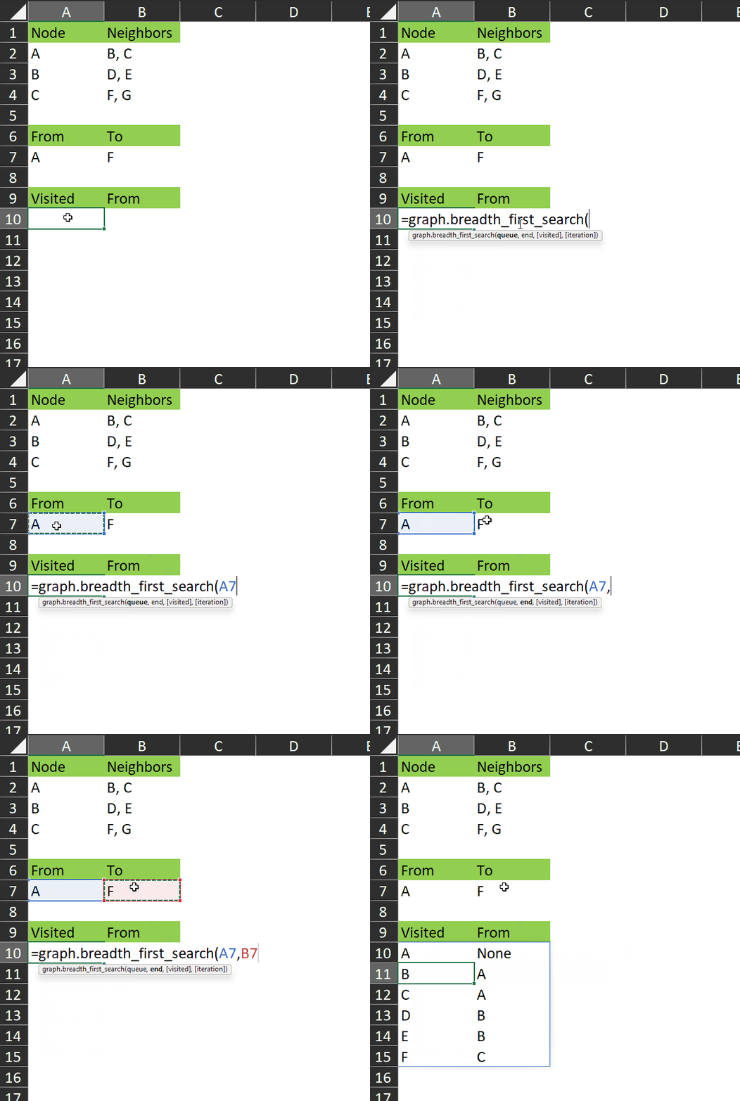
This may not seem very useful with such a small dataset, but consider a much more complex graph with hundreds of nodes and many different paths between each node. This algorithm will find the shortest path between any two nodes. 

But we don’t need to stop there. Let’s look next at a function to extract the path from the visited array.

graph.get_path

get_path = LAMBDA(start, next, search_function, [visited], [path],
    LET(
        _visited, IFOMITTED(visited, search_function(start, next)),
        _step, FILTER(_visited, TAKE(_visited, , 1) = next),
        _path, IFOMITTED(path, _step, VSTACK(_step, path)),
        //_path, IF(ISOMITTED(path), _step, VSTACK(_step, path)),
        _next, INDEX(_step, 1, 2),
        _result, IF(
            _next = start,
            CHOOSECOLS(_path, {2, 1}),
            graph.get_path(start, _next, search_function, _visited, _path)
        ),
        _result
    )
);

This function takes three required parameters:

1. start – which is the “from” node in a search.
2. next – when we call from the spreadsheet, this parameter is passed the “to” node – the node being searched for. Because this function recursively traverses a visited array starting at the end node, the end node is considered the “next” node to find in the visited array when we start. As the function recurses, the “next” node is the node that each node was visited from. In this way, we move through the visited array until we reach the start node. 
3. search_function – this get_path function is designed to accept any of a number of functions (I have also written a graph.depth_first_search lambda). So in the context of this article, the value passed to this parameter is the graph.bread_first_search function. 

And two optional parameters, which are used by the recursion:

1. [visited] – this is created by a call to the search function (graph.breadth_first_search in this context) and is passed through each iteration in order to be able to find the path from the end back to the start.
2. [path] – as each “visited from” node is encountered, those rows from the [visited] array are added to this [path] array in preparation for returning this [path] array as the result of this function.

It works like this:

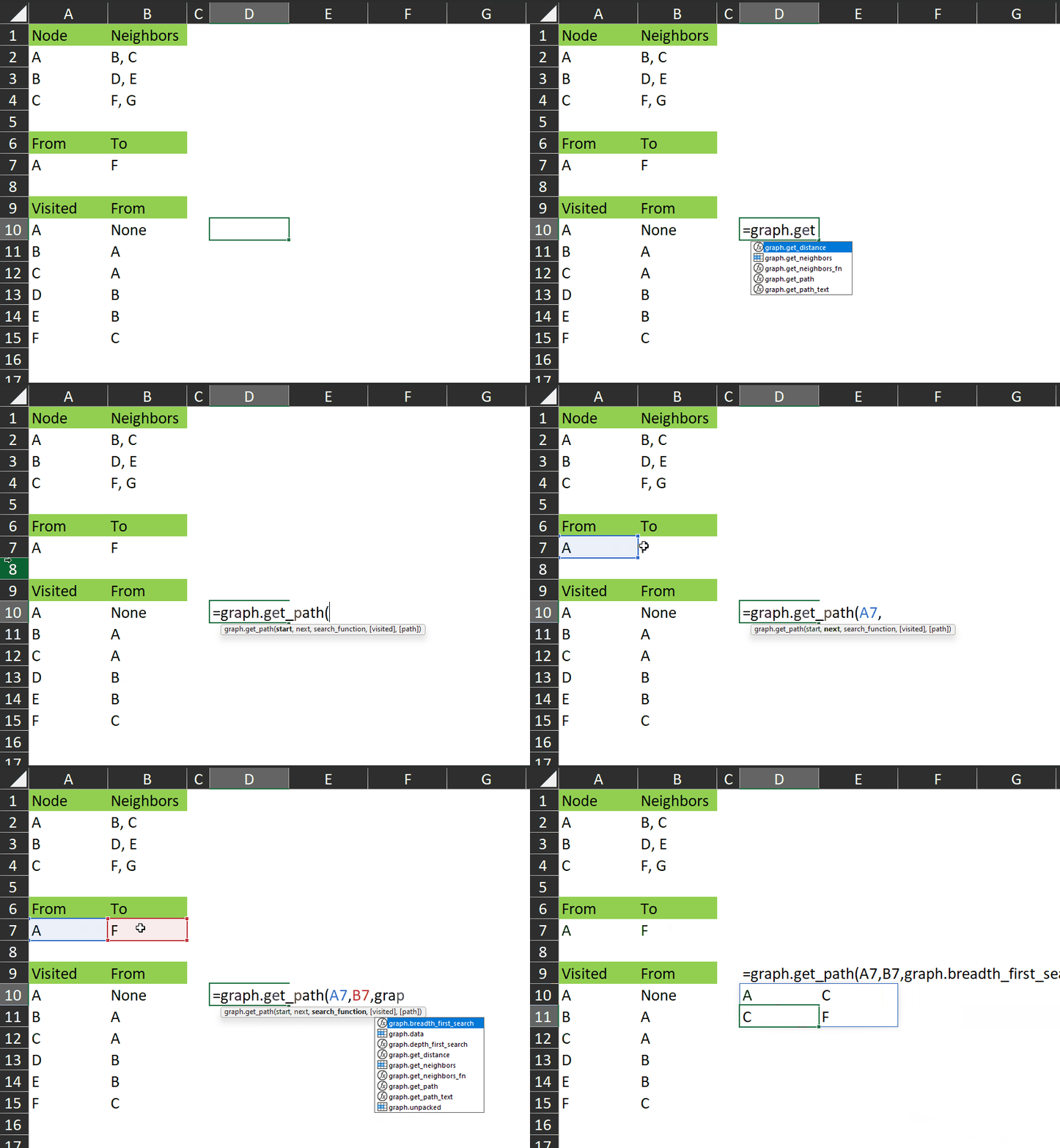
You can see it returns those rows from the visited array that represent the shortest path between A and F. 

• _visited – here we’re using IFOMITTED to initialize the visited parameter with the result of the search according to whatever search_function was passed to get_path. In the gif above, I’ve passed graph.breadth_first_search as the search function, so the value put into _visited is the array returned by that function – i.e. the data shown in cells A10:B15 in the gif above. 
• _step – we filter the _visited array for the next node. 
• _path – if the [path] parameter is omitted – i.e. it’s the first iteration – then initialize _path with _step (that row from _visited containing the end node), otherwise stack _step on top of [path].
• _next – get the node from which we arrived at the current node. This is the value in column 2 of the _step variable (which is the row from the _visited array that contains the “next” node).
• _result – if _next is equal to start, then return the path, with the columns switched so that “from” is in the first column and “to” is in the second column. This is so that the path makes more sense and reads from left to right, top to bottom. If they aren’t the same, then iterate graph.get_path, passing start, _next, search_function, _visited and _path into the next iteration, which then looks for the next node and causes the function to recurse until the start node is arrived at. 

I hope that makes sense. 

The next function offers a way to show the path in a more friendly way.

graph.get_path_text

get_path_text = LAMBDA(start, end, search_function,
    LET(
        _path, graph.get_path(start, end, search_function),
        TEXTJOIN(" " & UNICHAR(10132) & " ", TRUE, UNIQUE(TOCOL(_path)))
    )
);

It works like this:

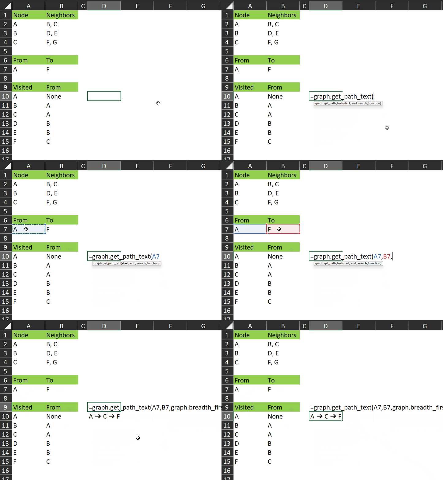
As you can see, it gives us a single value which clearly shows the nodes visited between the start and end. 

It takes three required parameters, which are the same as graph.get_path. The function calls graph.get_path to return the path between the nodes (as described above), then converts the path array to a column using TOCOL, takes the UNIQUE items from that column and joins them with this unicode array character, inserted with UNICHAR(10132). 

Just one last function for now! 

graph.get_distance

get_distance = 
    LAMBDA(from, to, search_function,
        LET(
            _path, graph.get_path(from, to, search_function),
            ROWS(_path)
        )
    );

As you can see, this function returns the number of rows in the return array of graph.get_path. This is the number of edges traversed between the start and end nodes of a path.

In summary

We saw how to perform a breadth-first search using Excel.

Using recursive lambda functions, we traversed data that represents the nodes and edges of a graph and returned the visited nodes, the shortest path in two formats, and the distance between two given nodes. 

I hope this post has been useful to you. You are welcome to take the code from the gist linked at the top of this page. 

Do you have any ideas how this can be improved? Please let me know in the comments or connect with me on LinkedIn or on @flexyourdata on YouTube.