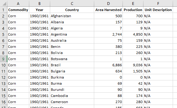
I downloaded some data from the USDA FAS custom query builder. The file contains the area harvested of corn in many harvest years for non-US countries.
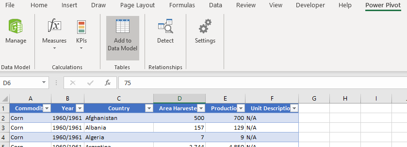
I want to calculate the % of non-US corn area that each country represents in the latest two full harvest years and then calculate the change in percentage points between those two years. The downloaded data looks like this:
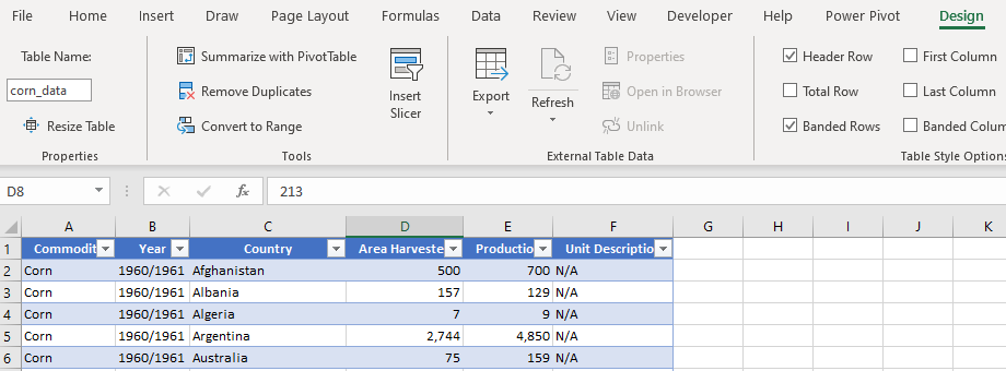
I’m going to use the harvest years “2017/2018” and “2018/2019”. The first thing I’ve done is format the data as a table, by selecting anywhere in the data and pressing Ctrl+T, then I’ve given the table the name “corn_data” in the Table Name box in the Properties group on the Design tab in the Table Tools group on the ribbon.
The formatted table looks like this:
So, I said I want to calculate the % of non-US corn area that each country represents in the latest two full harvest years and then calculate the change in percentage points between those two years.
I can create a pivot table that looks like this:
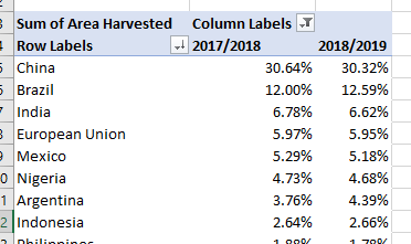
To do that, I’ve put Area Harvested in the values area of the pivot table and changed the “Show values as” to “% of Column Total”.
I want to calculate for each row the difference for between the percentage for 2017/2018 and 2018/2019. Unfortunately, because I’ve already used “Show values as” to calculate the “% of Column Total”, I can’t use “Show values as” again to calculate the difference between the percentages!
I’ll probably have to put a simple formula in the next column, like this:
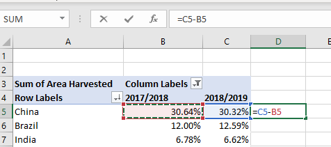
Simple enough, but not very flexible. If the pivot table changes shape (I add more columns), or I add too many filters, the formula will quickly get messed up and I’ll have to tweak it to keep it working.
Luckily, there’s a way to do both using PowerPivot. To get started, I’m going to add my formatted Table to the PowerPivot Data Model by clicking “Add to Data Model” on the PowerPivot tab on the ribbon.
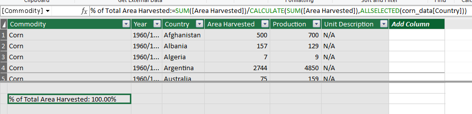
After I do that, I’m going to create a measure in PowerPivot that calculates the “% of Column Total”. I type this formula into the calculation area (that grid at the bottom):
SUM([Area Harvested])/CALCULATE(SUM([Area Harvested]),ALLSELECTED(corn_data[Country]))
I’ve given the measure the name “% of Total Area Harvested” and set the default format to percentage with 2 decimals.
in the PowerPivot window, it looks like this:
To break that formula down a little, we’re just taking the sum of the area harvested, which is going to be the sum in the pivot table on each row (for each country), and dividing it by the sum of the area harvested over all of the selected countries.
We use the CALCULATE function to tell the measure to change the context from the row of the pivot table to the items specified in the second parameter. In this case, we want the sum of the area harvested for all of the filtered countries.
ALLSELECTED just defines that set of data as the filtered countries in the pivot table. If we wanted to calculate the sum of the area over all countries, even if we had filtered some out of the pivot table, we’d change that ALLSELECTED function to ALL.
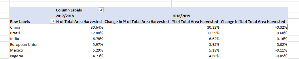
Anyway, after creating a pivot table from the Power Pivot window, we can use the measure like this:
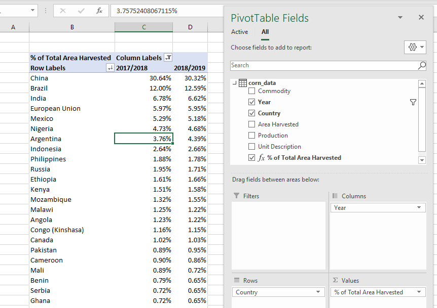
You can see it’s produced the same result as the pivot table at the top of this post.
So what?
Well, the difference is that now I can change the “Show values as” for the new measure to “Difference from” and select “Year” and “(previous)” to get the difference calculation I was after, but embedded in the Pivot Table. So now, if I add extra years, or filters, I won’t have to spend time messing about with formulas!