-
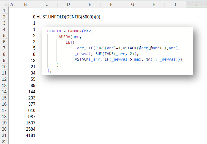
Unfold a list with this new function
In this post you’ll learn to unfold a list from a value with a recursion wrapper called LIST.UNFOLD. INTRODUCTION In Excel as in many other languages, we can use REDUCE to reduce (or fold) a list into a single value. We iterate over the list, and at each element apply a function. The result of […]
-
Format A Row Of Data For SQL INSERT
The gist for this lambda function can be found here. If you sometimes need to quickly put some Excel data into a SQL table or use the data in a CTE, you may have found yourself doing something like this: Here’s a LAMBDA I’ve called SQLVALUES: =LAMBDA(t,LET(d,IFS(ISTEXT(t),”‘”&SUBSTITUTE(t,”‘”,”””)&”‘”,ISBLANK(t),”NULL”,LEFT(MAP(t,LAMBDA(x,CELL(“format”,x))),1)=”D”,TEXT(t,”‘YYYY-MM-DD HH:mm:ss’”),TRUE,t),”(“&TEXTJOIN(“,”,FALSE,d)&”)”)) This will: Wrap the tuple in parentheses […]
-
Split An Alphanumeric String Into An Array Of Characters
=LAMBDA(rng,vertical,LET(chars,MID(rng,SEQUENCE(LEN(rng)),1),IF(vertical,chars,TRANSPOSE(chars)))) This LAMBDA function takes two arguments: rng – a cell containing a text string vertical – TRUE/FALSE. If TRUE, the LAMBDA will return a vertical array of the characters in rng. If FALSE, the LAMBDA will return a horizontal array of the characters in rng In my file, I have named this LAMBDA “CHARACTERS”. […]
-
Filter Out Rows With Empty Cells
If you want to quickly get all rows which don’t have any blanks in any columns, you can combine FILTER, BYROW and AND, like this: =FILTER(range,BYROW(range,LAMBDA(r,AND(r<>””)))) Here, I’ve defined a LAMBDA function, which is really just a way of applying some logic (in the second parameter) to some data (in the first parameter). I have […]
-
Excel: Calculate The Difference Between “Percentage Of Column Total” Columns
I downloaded some data from the USDA FAS custom query builder. The file contains the area harvested of corn in many harvest years for non-US countries. I want to calculate the % of non-US corn area that each country represents in the latest two full harvest years and then calculate the change in percentage points […]
-
Excel: Use Names To Make Your Formulas Easier To Read
There’s a useful but under-used feature in Excel that can make your formulas much easier to read and understand. In the image below, the Name Box is the white box where it says A2. You can see that I have an Important Value in cell A2. I’m going to use that value all over my […]