excel-lambda-FORECAST.ETS.COMPARE – Build a forecast for comparison with actuals with a single formula

The gist for this lambda function can be found here.

Forecasting in Excel

Excel comes with several functions that allow us to quickly produce forecasts on time-series datasets.

Data>Forecast Sheet

One method you can use is the “Forecast sheet” button which can be found on the “Data” tab of the ribbon in Excel versions 2016 onwards. For a primer on what that does and how it works, I encourage you to watch this video.

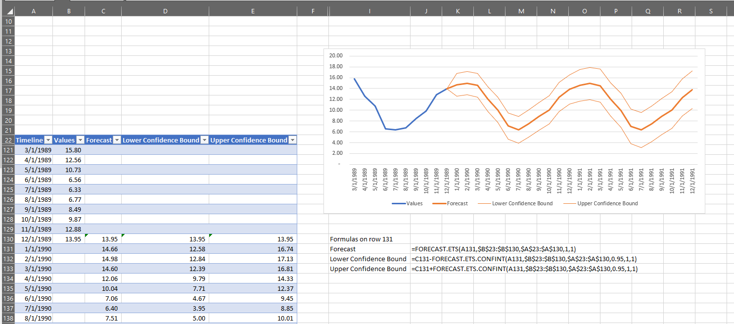
The “Forecast sheet” button uses the FORECAST.ETS function to produce a table where the original values are in one column and the forecast values are in an adjacent column.

The “Forecast” column does not include the actual values in non-forecasted rows.

Additionally, it does not consider scenarios where we might have actuals for the rows we are forecasting. As such, the “Values” column does not have any comparative data in the forecast rows.

You can see that “Forecast sheet” also creates a chart and can optionally show confidence boundaries for the forecast values.

I want to be able to quickly use a forecast as an additional quality control check on my time series data of temperatures in Melbourne in the 1980s. To do this, I need to be able to forecast rows I already have data for using the other rows. Because of this, “Forecast sheet” is not going to help.

If you’ve not used the “Forecast sheet” button before, I encourage you to watch the video I linked above but I would also urge caution in the use of such forecasts without a basic understanding of the algorithm and its limitations.

FORECAST.ETS does not perform well when considering long-range forecasts

=FORECAST.ETS

The FORECAST.ETS function uses what is known as AAA exponential smoothing to calculate forecasts.

The three As in the name represent the Addition to the model of terms for:

1. residuals
2. trend
3. seasonality

It’s my understanding that FORECAST.ETS has the Holt-Winters exponential smoothing algorithm at its core.

Since that algorithm requires selection of several parameters – alpha, beta and gamma – and no such arguments are present in the Excel function, I can only assume there is some proprietary optimization happening behind-the-scenes to select values for those parameters that produce what Excel considers a “best” forecast for the data.

Enter FORECAST.ETS.COMPARE

I want to build a lambda that will take the FORECAST.ETS function and wrap it in some additional logic so that the output includes a comparison between actuals and forecast as well as variances between the two for each forecasted period.

I want to use the forecast as a quality control check against my actuals.

If they deviate too far from each other, this may indicate a problem with my data pipeline or in my assumptions about the collected data.

If you’d like to experiment with the same dataset, here’s the PowerQuery I used to gather temperatures in Melbourne in the 1980s:

let
    Source = Csv.Document(Web.Contents("https://raw.githubusercontent.com/jbrownlee/Datasets/master/daily-min-temperatures.csv"),[Delimiter=",", Columns=2, Encoding=65001, QuoteStyle=QuoteStyle.None]),
    #"Promoted Headers" = Table.PromoteHeaders(Source, [PromoteAllScalars=true]),
    #"Changed Type" = Table.TransformColumnTypes(#"Promoted Headers",{{"Date", type date}, {"Temp", type number}}),
    #"Inserted Start of Month" = Table.AddColumn(#"Changed Type", "Start of Month", each Date.StartOfMonth([Date]), type date),
    #"Grouped Rows" = Table.Group(#"Inserted Start of Month", {"Start of Month"}, {
        {"average_temp", each List.Average([Temp]), type nullable number}, 
        {"min_temp", each List.Min([Temp]), type nullable number}, 
        {"max_temp", each List.Max([Temp]), type nullable number}})
in
    #"Grouped Rows"

The query produces a dataset where each row represents the mean, min and max temperature in one month in the 1980s. You can paste it into the Advanced Editor of a blank query in Power Query in Excel.

In the example below, I’ll use the new lambda function to calculate forecasts for arbitrary numbers of months at the end of that time series

This is the definition of FORECAST.ETS.COMPARE

=LAMBDA(data,
        dates_in_column,
        values_in_column,
        forecast_last_x_values,
        [seasonality],
        [data_completion],
        [aggregation],
  LET(
    _data,data,
    _data_rows,ROWS(_data),
    _data_cols,COLUMNS(_data),
    _dates,INDEX(_data,,dates_in_column),
    _values,INDEX(_data,,values_in_column),
    _train_end_row,_data_rows-forecast_last_x_values,
    _dates_train,INDEX(_dates,1,1):INDEX(_dates,_train_end_row,1),
    _values_train,INDEX(_values,1,1):INDEX(_values,_train_end_row,1),
    _header,{"dates","actuals","forecast","variance","variance %"},
    _array,
    MAKEARRAY(
      _data_rows+1,
      _data_cols+3,
      LAMBDA(r,c,
        LET(
          _row_date,INDEX(_dates,r-1,1),
          _row_value,INDEX(_values,r-1,1),
          _forecast,FORECAST.ETS(
                      _row_date,
                      _values_train,
                      _dates_train,
                      IF(ISOMITTED(seasonality),1,seasonality),
                      IF(ISOMITTED(data_completion),1,data_completion),
                      IF(ISOMITTED(aggregation),0,aggregation)
                    ),
          _var,_forecast-_row_value,
          _var_pct,_forecast/_row_value-1,
          IFS(
            r=1,INDEX(_header,1,c),
            c=1,_row_date,
            c=2,_row_value,
            r-1<=_train_end_row,CHOOSE(c-2,_row_value,0,0),
            r-1>_train_end_row,CHOOSE(c-2,_forecast,_var,_var_pct),
            TRUE,NA()
          )
        )
      )
    ),
    _array
  )
)

This is how it works:

As you can see, the accuracy of the forecast suffers if we try to forecast too many months, so it bears repeating:

FORECAST.ETS does not perform well when considering long-range forecasts

The lambda has four required arguments:

1. data – this is a two-column range or array of data where one of the columns contains dates and one of the columns contains the values to be used as the basis for the forecast
2. dates_in_column – is an integer, either 1 or 2, telling the function which of the two selected columns in data contains the dates
3. values_in_column – is an integer, either 1 or 2, telling the function which of the two selected columns in data contains the values to be used as the basis for the forecast
4. forecast_last_x_values – is an integer which is smaller than the total number of rows in data. This value is the number of periods at the end of the selected data range that you would like to create forecasts for based on all the other rows not in the last X rows

There are also three optional arguments, which are used to control FORECAST.ETS. These are used in exactly the same way as in that function, and I include here the description of those arguments copied from the support page:

5. seasonality – The default value of 1 means Excel detects seasonality automatically for the forecast and uses positive, whole numbers for the length of the seasonal pattern. 0 indicates no seasonality, meaning the prediction will be linear. Positive whole numbers will indicate to the algorithm to use patterns of this length as the seasonality. For any other value, FORECAST.ETS will return the #NUM! error. Maximum supported seasonality is 8,760 (number of hours in a year). Any seasonality above that number will result in the #NUM! error.
6. data_completion – Although the timeline requires a constant step between data points, FORECAST.ETS supports up to 30% missing data, and will automatically adjust for it. 0 will indicate the algorithm to account for missing points as zeros. The default value of 1 will account for missing points by completing them to be the average of the neighboring points
7. aggregation – Although the timeline requires a constant step between data points, FORECAST.ETS will aggregate multiple points which have the same time stamp. The aggregation parameter is a numeric value indicating which method will be used to aggregate several values with the same time stamp. The default value of 0 will use AVERAGE, while other options are SUM, COUNT, COUNTA, MIN, MAX, MEDIAN

It’s important to note that the FORECAST.ETS function expects the date values in the dates column to be equally spaced (i.e. one row per day, or per week, or per month, etc) and though it will try to adjust for up to 30% gaps in the timeline, it’s recommended that you avoid having gaps.

While FORECAST.ETS doesn’t require the timeline (dates) to be sorted, FORECAST.ETS.COMPARE does, so please ensure that the data selected is sorted in ascending date order before using.

How it works

Let’s break it down. First, we use LET to create some variables and perform some simple calculations.

  LET(
    _data,data,
    _data_rows,ROWS(_data),
    _data_cols,COLUMNS(_data),
    _dates,INDEX(_data,,dates_in_column),
    _values,INDEX(_data,,values_in_column),
    _train_end_row,_data_rows-forecast_last_x_values,
    _dates_train,INDEX(_dates,1,1):INDEX(_dates,_train_end_row,1),
    _values_train,INDEX(_values,1,1):INDEX(_values,_train_end_row,1),
    _header,{"dates","actuals","forecast","variance","variance %"},

• _data – this is just a renaming of the function argument “data“. As a rule, I am trying to prefix variables internal to the lambda with an underscore to avoid confusion
• _data_rows – this is the count of the rows in _data
• _data_cols – this is the count of the columns in _data (must be 2!)
• _dates – here, we use INDEX to return the column from _data that corresponds to the argument dates_in_column
• _values – here, we use INDEX to return the column from _data that corresponds to the argument values_in_column
• _train_end_row – we subtract the value from the argument forecast_last_x_values from the variable _data_rows to determine the last row of data that contains values that we won’t create a forecast for
• _dates_train – here we use the reference form of INDEX (note the colon between the two INDEX calls) to return the rows from row 1 of the _dates variable (which represents all the dates in the data) to row _train_end_row. These are the dates that will be passed into the timeline argument of the FORECAST.ETS function
• _values_train – here we use the reference form of INDEX (note the colon between the two INDEX calls) to return the rows from row 1 of the _values variable (which represents all the values in the data) to row _train_end_row. These are the values that will be passed into the values argument of the FORECAST.ETS function
• _header – here we are defining a typed array as the header for the output array

Next, we build the output array:

MAKEARRAY(
      _data_rows+1,
      _data_cols+3,
      LAMBDA(r,c,
        LET(
          _row_date,INDEX(_dates,r-1,1),
          _row_value,INDEX(_values,r-1,1),
          _forecast,FORECAST.ETS(
                      _row_date,
                      _values_train,
                      _dates_train,
                      IF(ISOMITTED(seasonality),1,seasonality),
                      IF(ISOMITTED(data_completion),1,data_completion),
                      IF(ISOMITTED(aggregation),0,aggregation)
                    ),
          _var,_forecast-_row_value,
          _var_pct,_forecast/_row_value-1,
          IFS(
            r=1,INDEX(_header,1,c),
            c=1,_row_date,
            c=2,_row_value,
            r-1<=_train_end_row,CHOOSE(c-2,_row_value,0,0),
            r-1>_train_end_row,CHOOSE(c-2,_forecast,_var,_var_pct),
            TRUE,NA()
          )
        )
      )
    ),
    _array
  )
)

The output array will be the same size as the input data, with an additional row for the header.

It will have the same number of columns as the input data (2) plus 3 additional columns:

1. “Forecast” for the copy of the values that has forecasted values in the last forecast_last_x_values rows
2. “Variance” for the difference between the forecast and the actuals
3. “Variance %” for the variance expressed as a percentage change from the actuals

The lambda function used in MAKEARRAY must have two arguments – row and column. I have called them r and c.

Next, we are using LET to define the various elements of each row:

• _row_date – we get the value from the _dates variable of the row that corresponds to r-1 in the output array. We must use r-1 because the output array is shifted one row down from the input array because of the header
• _row_value – similarly, we get the value for the current row from the _values variable
• _forecast – here, we call the FORECAST.ETS function using
  • _row_date as the Target date argument,
  • _values_train as the values argument. Remember: this variable contains only those rows up to and including the row just before the last X values as defined by forecast_last_x_values
  • _dates_train as the timeline argument. Similarly, this contains the dates up to and including the row just before the last X values as defined by forecast_last_x_values 
  • If we have passed a seasonality argument to FORECAST.ETS.COMPARE, we pass it onward to FORECAST.ETS, otherwise we use 1, which tells the function to automatically determine a value for seasonality
  • If we have passed a data_completion argument to FORECAST.ETS.COMPARE, we pass it onward to FORECAST.ETS, otherwise we use 1, which tells the function to complete missing points in the dates series by taking the average of neighboring points. This will work for up to 30% missing points. Nevertheless, for better results I encourage you to ensure that your date series passed into the forecast doesn’t have missing points
  • If we have passed an aggregation argument to FORECAST.ETS.COMPARE, we pass it onward to FORECAST.ETS, otherwise we use 0, which tells the function to use the average function to deal with duplicate time series entries in the list of dates
• _var – is the _row_value subtracted from the _forecast
• _var_pct – is the percentage change that the _forecast represents from the _row_value

Finally, we use IFS to put the right variables in the correct cells in the output array:

• If the row is 1, place the header in the output array
• If the column is 1, place the date in the output array
• If the column is 2, place the original values in the output array
• Otherwise,
  • If the row is less than or equal to the last row of non-forecasted data (_train_end_row), then put the _row_value in column 3 (Forecast) and zero in columns 4 and 5 (the variance columns)
  • If the row is greater than the last row of non-forecasted data, then put the _forecast in column 3 and the variance and variance pct in columns 4 and 5
• Otherwise, return #N/A

Finally, we tell LET to return _array to the calling lambda and from there back to the spreadsheet. I find it useful to name the result of MAKEARRAY like this rather than simply having it as the last argument of LET; this let’s me quickly switch between outputs as I’m developing and testing the lambda.

In conclusion

Excel has several built-in tools to help you create forecasts on time-series data.

We can use lambda functions to embed those forecasting tools into a format that is useful for our needs.

In this example, I created a lambda that allows comparison of forecast vs. actuals.

Do you have any repetitive tasks in Excel you wish were simpler? Drop a comment below and let’s see if we can figure it out together!