-
UPDATE! 🪲 How to make a timestamp column for an Excel Table
I’m reliably informed by a man on the inside that the capability described below, tantalizing though it may be, is in fact the side effect of a bug! And like many bugs, it will soon be squashed. Flattened. Smooshed out of existence. So be warned! Full credit for the idea in this post goes to Lorimer Miller. I don’t know how he comes across these ideas, but I’m glad he does. Let’s get into it. A reminder about volatility You may have heard about certain Excel functions being volatile. Among them are INDIRECT, OFFSET, NOW, TODAY, RAND and RANDARRAY. There…
-
Use XLOOKUP and XMATCH with regular expressions (regex)
The Excel team introduced support for regular expressions in May 2024 with three new functions The functions were announced in this post on the Microsoft 365 Insiders blog. As well as these new functions, we learned that we will be able to use regular expressions with XLOOKUP and XMATCH in the near future. Regex coming soon to XLOOKUP and XMATCH We will also be introducing a way to use regex within XLOOKUP and XMATCH, via a new option for their ‘match mode’ arguments. The regex pattern will be supplied as the ‘lookup value’. This will be available for you to…

-
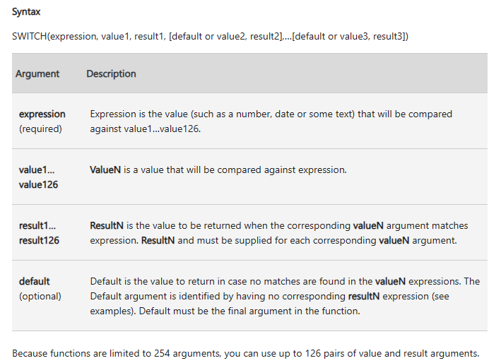
The SWITCH and LET functions – Excel formula performance
Let me get right to the point. Both SWITCH and unused complex names in LET can slow down your formulas Introduction This formula returns a large array: In the Beta version of Excel I’m using, the above formula can be written like this: I’ll use the shorter version for the remainder of this post. This MAKEARRAY formula creates an array of 10000 rows and 1000 columns. For each cell in the array, it uses the PRODUCT function to multiply the row number by the column number. It takes my computer about 3 seconds to return this formula. By most measures,…