I’m reliably informed by a man on the inside that the capability described below, tantalizing though it may be, is in fact the side effect of a bug! And like many bugs, it will soon be squashed. Flattened. Smooshed out of existence. So be warned!
Full credit for the idea in this post goes to Lorimer Miller. I don’t know how he comes across these ideas, but I’m glad he does.
Let’s get into it.
A reminder about volatility
You may have heard about certain Excel functions being volatile. Among them are INDIRECT, OFFSET, NOW, TODAY, RAND and RANDARRAY. There are a few others. You can read about volatile functions in this article on Microsoft Learn.
From that article:
A volatile function is always recalculated at each recalculation even if it does not seem to have any changed precedents. Using many volatile functions slows down each recalculation, but it makes no difference to a full calculation.
But let’s restrict ourselves to talking about NOW, for now.
NOW
As mentioned in the documentation, NOW:
Returns the serial number of the current date and time.
This is great, but because NOW is volatile, it updates every time pretty much anything happens in the workbook. Take a look at what happens if we try to use =NOW() as a formula for a Timestamp column in a Table.
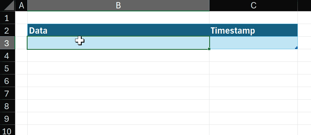
It’s pretty easy to see that if we want to track the time when a row is added to a Table, this isn’t going to work.
And here’s where Lorimer’s amazing find comes into play.
Dereferenced non-volatile NOW
Woah, what a heading. But it’s really not that complicated. Just take a look at this revised formula in the Timestamp column and then watch as new rows are added:
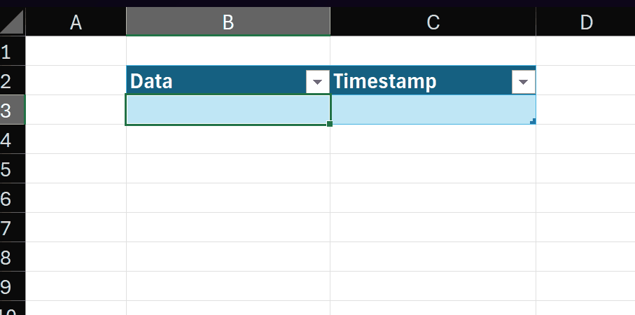
As new rows are added, the timestamps in the earlier rows don’t change!
I don’t know about you, but when I first saw this, I was 🤯 and not a little 😲.
But, surely this can’t be that easy? Surely there’s a catch? Well… yes. As mentioned in the latter rows of the gif above, we have to be careful if we want those timestamps to stay the same.
I’ve tested a few things and found two shortcuts that will recalculate those NOW values. According to the article I linked above:
You can force a full calculation of all the formulas by pressing Ctrl+Alt+F9, or you can force a complete rebuild of the dependencies and a full calculation by pressing Shift+Ctrl+Alt+F9.
Note that both of these act on all open workbooks. So if you do choose to use this method, you should definitely not use those shortcuts. In VBA, these behaviors are accessed with Application.CalculateFull (for Ctrl+Alt+F9) and Application.CalculateFullRebuild (for Shift+Ctrl+Alt+F9). But I would hazard a guess that if you are using those commands in VBA, you probably don’t need or want a formula for a timestamp. It’s much better, in that case, to calculate the current date and time in VBA and write it to the workbook.
But for all the rest of us, this approach could be useful! Here it is again, for reference:
=(@NOW)()
But it doesn’t end there.
Why “de-referenced”?
To be 100% honest, I don’t fully understand why this works, but here’s my guess. The @ operator is the implicit intersection operator. While it has a long explanation, what it does to arrays is interesting. It essentially takes the top-left cell of any array and converts it into a scalar value.
And it’s this behavior which I believe is “de-referencing” – not a reference in terms of a place in a workbook, but a reference to the function in the calculation chain. It’s turning that function into a scalar object – and then passing that scalar – which is a function – as an eta-reduced LAMBDA function into the formula.
In this way, I think the calculation engine doesn’t consider this formula to be part of the volatile things that need to be updated regularly.
That’s my take, but I am ready to be corrected on that in the comments!
But nevermind all that, let’s take a look at…
Another volatile function, de-volatilized (is that a word? It is now)
Since this works with NOW, you might also wonder if it works with other volatile functions. And it does!
A common task might be to create an array of random numbers between two values. And the normal approach here is to use RANDARRAY, then copy and paste values the result (because if you don’t, the random numbers change every time anything else in the workbook changes – which can be problematic).
Take a look at what happens if we wrap the de-referenced function in the same way:
=(@RANDARRAY)(10,1,1,100,TRUE)
As you can see, even when we add data to the sheet, or perform calculations on the random array, the array doesn’t change.
Again, this is subject to the same limitations on the shortcuts I mentioned above. Here’s a summary of the tests I performed and what happened to the =(@NOW)() formulas.
| Action | Recalculated =(@NOW)() | Added to this table |
|---|---|---|
| Adding a row to a Table | No | 2025-05-29 |
| Saving and reopening | No | 2025-05-29 |
| F9 (recalculate sheet) | No | 2025-05-29 |
| Ctrl+Alt+F9 | Yes | 2025-05-29 |
| Ctrl+Shift+Alt+F9 | Yes | 2025-05-29 |
| VBA: Application.Calculate | No | 2025-05-29 |
| VBA: CalculateFull | Yes | 2025-05-29 |
| VBA: CalculateFullRebuild | Yes | 2025-05-29 |
| Calling a volatile VBA UDF | No | 2025-05-29 |
| Using “Refresh All” | No | 2025-05-30 |
| Deleting a Table row | Yes | 2025-05-30 |
| Inserting a Table row (not the same as adding at the bottom) | Yes | 2025-05-30 |
| Deleting a Sheet row/column | Yes | 2025-06-02 |
| Inserting a Sheet row/column | Yes | 2025-06-02 |
I will add items to this table as I become aware of them. If you run your own tests and find some behavior that recalculates this kind of formula, please let me know and I’ll add it to the table.
In summary, I do not warranty anything here. I don’t say you should do this, I’m just saying you can!
Want to learn how to build a recursive LAMBDA function that calculates the Levenshtein distance between two text strings? Take a look at this.
Leave a Reply