This is my attempt to answer a question I have asked myself many times over the last few months: What is a thunk in an Excel lambda function?
Background
Many of the new dynamic array functions that create arrays, such as MAKEARRAY, SCAN, REDUCE and so on, will not allow an element of the array created to contain an array.In short, an array of arrays is not currently supported.
As an example, consider the SCAN function. The description on the support site says
Scans an array by applying a LAMBDA to each value and returns an array that has each intermediate value
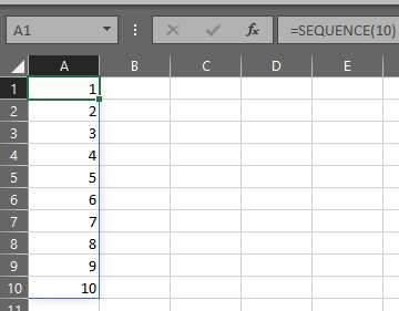
To show you what this means, consider the array of 10 integers created by SEQUENCE(10):
Scan takes this form:
=SCAN ([initial_value], array, lambda(accumulator, value))
A very simple SCAN function can iterate through each item in that array of 10 integers and apply some function to it.
The function that’s used as the third parameter is commonly seen like this:
LAMBDA(a,b,(some calculation involving a, b or both))
Where a is the “accumulator”, which is another way of saying it’s the result from this function during the previous iteration (the previous row of the array), and b is the value in the current row of the array passed in to scan.
The initial_value is there so that the accumulator can be given a value during the first iteration.
To see how this works, let’s look at a simple example:
=SCAN(0,A1#,LAMBDA(a,b,a+b))
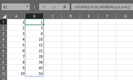
The initial_value for the accumulator a is zero. The array is the dynamic array in cell A1, which as we’ve seen is SEQUENCE(10), and the function is:
LAMBDA(a,b,a+b)
SCAN starts on on the first row of array. It sets a to be equal to the initial_value, which is zero. b is the value from row 1 of array, which in this example is 1. So, the function returns a+b=0+1=1 and the first output row is 1.
SCAN then moves to the next row. On row 2, a=(the result of the function from the prior row)=1, b=2, so a+b=1+2=3.
Similarly, on row 3, a=3, b=3, and a+b=6.
SCAN continues in this way until row 10, where a=45, b=10 and a+b=55, which of course is just the sum of the integers from 1 to 10.
So what does all this have to do with thunks? Well so far not much. Because we’ve only been using simple addition.
Things get complicated when the value we want to put in the output array is an array itself.
Enter arrays
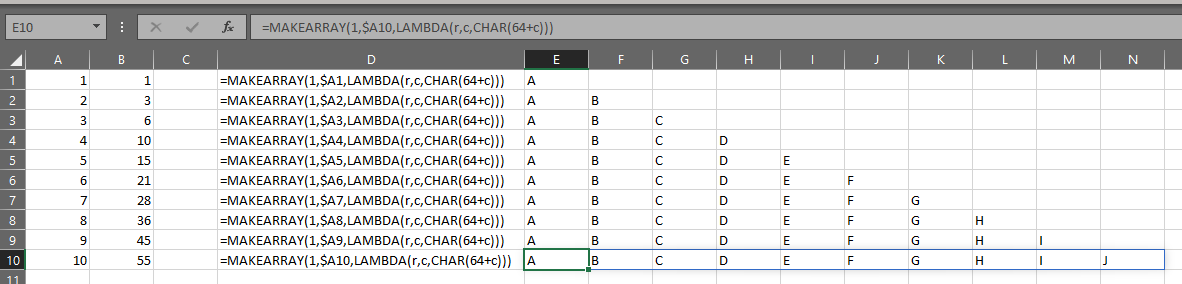
What if we wanted to use SCAN to create an array of arrays of letters for which each row has an array of 1 row and a number of columns determined by the value on the current row of SEQUENCE(10)?
The first row would have an array with 1 row and 1 column: {“A”}
The second row would have an array with 1 row and 2 columns: {“A”,”B”}
And so on.
We can create such a function on the first row and drag it down to the 10th row:=MAKEARRAY(1,$B26,LAMBDA(r,c,CHAR(64+c)))
The problem here is that SCAN does not allow for the result of an iteration to be an array. The result must be a value.
As you can see below, if we try to use this MAKEARRAY function inside the SCAN’s lambda function, it doesn’t work:
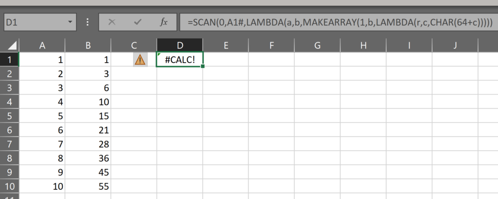
In the formula:
=SCAN(0,A1#,LAMBDA(a,b,MAKEARRAY(1,b,LAMBDA(r,c,CHAR(64+c)))))
The calculation in the lambda function within SCAN is the MAKEARRAY function. Unsurprisingly, it makes an array. The result of this lambda is, at each iteration, suppose to be assigned to the accumulator a. But since the result of this lambda is an array, it cannot be assigned to the accumulator, and so we get a #CALC! error.
It turns out that this problem of not being able to assign an array to an output of certain functions is quite common.Thunk to the rescue!
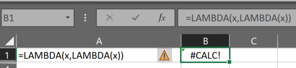
This is a thunk:
LAMBDA(x,LAMBDA(x))
It’s a lambda function with one parameter containing a lambda function with no parameters.
The parameter of the outer lambda – x – can be anything we want it to be. A text string, an integer, a decimal, a date, an array, another lambda function, anything.
This parameter is passed into the calculation section of the outer lambda. The calculation is a lambda, which I’m going to refer to as the inner lambda. This inner lambda has no parameters. Just a calculation.
The way we can think about this thunk is we pass a parameter into this outer lambda and it stores the parameter inside the inner lambda. It doesn’t do anything to it. Just puts it there and leaves it there for us to use later. This is particularly useful if that parameter happens to be a function itself, but we’ll get to that in another post.
What we need to remember right now is that it puts that parameter inside that inner lambda, and the inner lambda holds on to it.
Let’s take a look at this thunk thing.
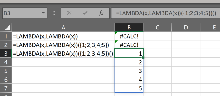
If we just use a plain thunk in a cell, it gives us a #CALC! error.
This is perhaps not surprising, as we know that when we use a lambda in a cell, we need to provide the parameters to that lambda in parentheses at the end of the formula. So let’s try that:
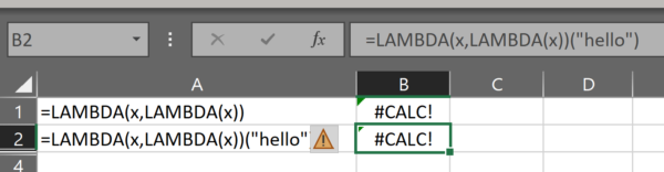
So we’ve provided a value for x – the parameter of the outer lambda. But it’s still returning a #CALC! error.
Well, yes and no. The truth is it’s showing us a #CALC! error, but hiding behind that error is the value LAMBDA(“hello”) – i.e. a parameter-less lambda function with a calculation equal to the value of the outer lambda!
Well, that’s great and all. But perhaps not immediately obvious why it’s of any use.
The thing about calling a lambda function is that you must complete the formality of providing the parentheses for the parameters – even if there are no parameters.
Look what happens when we add an open parenthesis and close parenthesis:
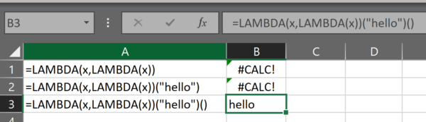
So we’ve got the parenthetical “hello” as the parameter to the outer lambda and for retrieving the value from the inner lambda, we have an empty parenthetical.
The effect of adding this empty parenthetical to the end of the formula is to evaluate the inner lambda and retrieve the value being stored in it. In this case, it’s just the word “hello”.
Let’s try it with an array.
We pass a 5-row array for the parameter x of the outer lambda: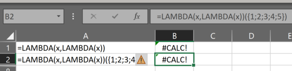
When we add the empty parenthetical, we get the array:
So, we can store this array in the inner lambda and retrieve it with this empty parenthetical.
This is where things start to get interesting.
Array of thunks
Let’s jump back to the 10-integer array.
What we’re going to do here is use our new found information about thunks to use SCAN to create an array of thunks.
=LET(
_thunk,LAMBDA(x,LAMBDA(x)),
_thunks,SCAN(0,$A$1#,LAMBDA(a,b,_thunk(MAKEARRAY(1,b,LAMBDA(r,c,CHAR(64+c)))))),
_thunks)
First, we’re using LET to define a single thunk. It’s just the same formula as described above. An outer lambda with a single parameter and inner lambda with no parameters.
Next, we’re using SCAN. We’re going to scan through the array in cell A1 again. Similarly to before, we’ll have zero as the initial_value and we’ll define that familiar lambda with parameters a and b. This time, however, we are going to take that MAKEARRAY function and use it as the parameter x of the thunk.
As we saw above, the thunk will take that MAKEARRAY function and put it inside the inner lambda, where it will be treated as a value.
Because it’s treated as a value, it can be used in the SCAN lambda. That “value” will of course return #CALC! for each row until we provide the empty parenthetical, so the result of this SCAN looks a lot like an array of #CALC! errors:
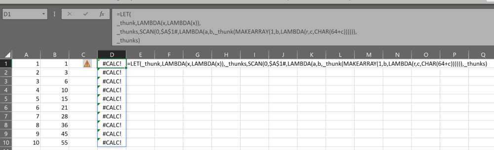
But remember, each one of those #CALC! errors is actually a single thunk. And each one of those thunks contains that MAKEARRAY function. And we can evaluate, or activate, that MAKEARRAY, by adding an empty parenthetical to the end of the formula.
Take a look at this:
=TRANSPOSE(LET(
_thunk,LAMBDA(x,LAMBDA(x)),
_thunks,SCAN(0,$A$1#,LAMBDA(a,b,_thunk(MAKEARRAY(1,b,LAMBDA(r,c,CHAR(64+c)))))),
INDEX(_thunks,10,1))())
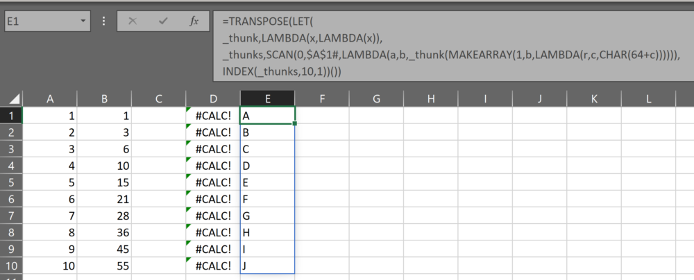
In this function, we’re using INDEX to get the 10th row from the array of thunks, then using the empty parenthetical to retrieve the array from the thunk, and finally wrapping the whole thing in TRANSPOSE. The result is a vertical array of the first 10 letters in the alphabet.
Again, not super useful yet. But now that we know how to get the array of letters from the 10th thunk, it’s just a few steps further to get ALL of the arrays from ALL of the thunks.
=LET(
_thunk,LAMBDA(x,LAMBDA(x)),
_thunks,SCAN(0,$B$26#,LAMBDA(a,b,_thunk(MAKEARRAY(1,b,LAMBDA(r,c,CHAR(64+c)))))),
_cols,MAX(SCAN(0,_thunks,LAMBDA(a,b,COLUMNS(b())))),
_out,MAKEARRAY(ROWS(_thunks),_cols,LAMBDA(r,c,INDEX(INDEX(_thunks,r,1)(),1,c))),
IFERROR(_out,""))
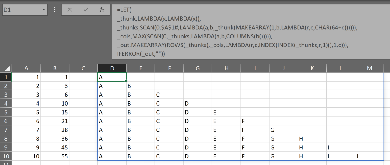
All that’s been done here is to build a rectangular array that is as wide as the widest array from the array of thunks. The array is then populated by each of the arrays in thunks in the array of thunks.
See where the empty parenthetical is? It’s attached to that inner call to INDEX. It’s there because that call to INDEX is grabbing a single element from _thunks, which is an array of thunks, which means that each element is a thunk and… you guessed it, we have to activate that thunk with the empty parenthetical.
The outer call to INDEX is then retrieving individual elements from each row’s array and placing them in the proper column in the output array.
In summary
So that’s it for this introduction to thunks and I hope it’s answered the question posed at the beginning of this post: “What is a thunk in an Excel lambda function?”
If you’d like to go away with a short answer to the question, try this:
A thunk is a parameter-less lambda where we can store complex values until we need them
Leave a Reply